Introduction
This topic introduces Bayesian statistical inference for a population proportion. We imagine a hypothetical population of two types which we will call "successes" and "failures". The proportion of successes in the population is denoted p. We take a random sample from the population -- we observe s successes and f failures. The goal is to learn about the unknown proportion p on the basis of this data.
A Model and Prior
In this setting, a model is represented by the population proportion p. We don't know it's value, and you represent your beliefs about its location in terms of a prior probability distribution. In this topic, we introduce proportion inference by using a discrete prior distribution for p.
You construct a prior by
specifying a list of plausible values for the proportion p
assigning probabilities to these values that reflect your knowledge about p
It is generally difficult to construct a prior since most of us have had little experience doing it. In the classroom setting, it is helpful to use standard types of prior distributions which are relatively easy to specify.
One type of standard "noninformative" prior
lets the proportion p be one of the equally spaced values 0, .1, .2, ..., .9, 1
assigns each value of p the same probability 1/11
This prior is certainly convenient and works reasonably well when you don't have a lot of data. But, as in the following example illustrates, it is relatively easy to construct a prior when there exists significant prior information about the proportion of interest.
An Example: Who's Better?
Suppose
that Andre Agassi is playing Boris Becker in a tennis match.
A model is a description of the relative abilities of Agassi and Becker.
You can use various expressions to describe models.
You might think the two
players "are evenly matched". Maybe
you're "sure Agassi will win", or maybe you think it is "likely, but not
a sure thing" that Becker will win. In
statistical inference, it is helpful if you can quantify these opinions.
Let p be the probability that Agassi wins.
One can view p as the proportion of times Agassi would win if the two
players could play a large number of tennis matches under identical conditions.
Next
you choose some plausible models, or values of the proportion p.
Suppose you think there are three possibilities --- Agassi is a little
better player than Becker, or they are evenly matched, or Becker is a little
better.
We
match these statements with the respective proportion values p = .6, .5, .4.
The value p = .6 is chosen by imagining about how many matches Agassi
would win against Becker in a series of 100 contests, if Agassi was indeed the
better player. The value p = .4 can be chosen in a similar way.
After you choose the models, you may think that some values of the proportion p are more or less likely. These opinions are reflected in a choice of prior probabilities on the set of models. For example, if you think Agassi will defeat Becker, then the proportion value p=.6 should get a larger prior probability that the value p = .4. Likewise, if you thought Becker was a better player, then p=.4 would get more probability. In the following discussion, we will illustrate inference for a person who thinks Agassi is the superior player and assigns the following prior to p:
| Prior | ||
| MODEL | p=.4 (Becker is better) |
.2 |
| p=.5 (same ability) |
.3 | |
| p=.6 (Agassi is better) |
.5 |
Likelihood
To use Bayes' rule, we next have to specify the likelihood. This is the probability of the actual data result for each model.
Here the data is the number of successes, s, and the number of failures, f, in our random sample taken from the population. Our model is the proportion of successes p. If the proportion is p, then the probability of observing s successes and f failures is
![]() .
.
Posterior Probabilities
Suppose that we have taken our sample and have observed values of s and f. By Bayes' rule, the posterior probability that the proportion takes on a value p is proportional to the product
![]()
where Prob(p) represents our prior probability of this value.
The calculation of the posterior probabilities is conveniently displayed using a tabular format (called the Bayes' table). (In the table below, p1, ..., pk represent k possible values of the proportion.)
| PROPORTION | PRIOR | LIKELIHOOD |
| p1 | P(p1) |
|
| p2 | P(p2) |
|
| pk | P(pk) |
|
To compute the posterior probabilities, we
multiply the prior and likelihood values for each proportion value to get products
sum the products
divide each product by the sum to get posterior probabilies
Computing the Posterior Probabilities for the Tennis Example
We illustrate computing the posterior probabilities in our example. Suppose Agassi and Becker play a single match and Agassi wins. So we have taken a single observation and we observed a success and so s = 1 and f = 0.
Here is the Bayes' table:
| p | PRIOR | LIKELIHOOD | PRODUCT | POSTERIOR |
| .4 | .2 | .4 | .2 x .4 =.08 | .08/.53 = .15 |
| .5 | .3 | .5 | .3 x .5 =.15 | .15/.53 = .28 |
| .6 | .5 | .6 | .5 x .6 =.30 | .30/.53 = .57 |
| SUM | .53 |
Before the tennis match, your probability that Agassi was better was .5. After seeing Agassi win the match, your new probability that Agassi is better has increased to .57. This means that you are now more confident that Agassi is better.
Computing Posterior Probabilities using a Bayes' box:
We
demonstrate the Bayes' box method computing the posterior probabilities.
This method helps in showing the connection between the model (value of p) and
the data (values of s and f). In
this example, suppose there are 300 pairs of tennis players just like Agassi (A)
and Becker (B). (The choice of 300
is made for convenience --- any large number divisible by 3 would be suitable.)
Your
prior placed probabilities .2, .3, .5 on the models "A is weaker than B", "A
and B are equally matched", "A is better than B".
So
you would expect 60 = 300 x .2 of the A's to be better than B's, 90 = 300 x .3 of the pairs to be
equally matched, and 150 = 300 x .5 B's would be
|
DATA |
||||
| Agassi wins | Becker wins | TOTAL | ||
| MODEL | p=.4 (Becker is better) |
60 | ||
| p=.5 (same ability) |
90 | |||
| p=.6 (Agassi is better) |
150 | |||
| TOTAL | 300 | |||
The
data in this example is the result of one tennis match.
There are two possible outcomes --- either "Agassi wins" or "Becker wins".
The
next step in this process is to relate the models to this data.
You
think about the frequencies of the data outcomes for each model.
Suppose p = .4 (Becker is a better player) and
Agassi and Becker play each other 60 times.
Then you would expect Agassi to win 24 matches and Becker the remaining
36. Similarly, if the players are equally good (p = .5) and
they play 90 matches, you expect each player to win 45 matches. If
Agassi is the superior player (p = .6) and they play 150 matches, then you expect Agassi to win
90 and
Becker 60. We place these counts in
a Bayes' box in which the row corresponds to a value of the proportion p and a
column is the result of the single tennis match.
|
DATA |
||||
| Agassi wins | Becker wins | TOTAL | ||
| MODEL | p=.4 (Becker is better) |
24 | 36 | 60 |
| p=.5 (same ability) |
45 | 45 | 90 | |
| p=.6 (Agassi is better) |
90 | 60 | 150 | |
| TOTAL | 300 | |||
Suppose
Agassi wins the match. Presumably
we would be more confident that Agassi is the better player.
We can learn how much more confident by updating our probabilities about
the models by use of Bayes' rule. This
computation is made by looking at the Bayes' box and restricting attention to
the observed data outcome ("Agassi wins match").
We note that Agassi won 24 + 45 + 90 = 159 matches in our hypothetical
experiment. Of these 159 matches,
Becker was the better player in 24 of them, the two players were equivalent in
45, and Agassi was better in 90. Our
updated table of model counts and proportions is given below.
|
DATA |
|||
| Agassi wins | PROPORTION | ||
| MODEL | p=.4 (Becker is better) |
24 | 24/159 = .15 |
| p=.5 (same ability) |
45 | 45/159 = .28 | |
| p=.6 (Agassi is better) |
90 | 90/159 = .57 | |
| TOTAL |
159 |
1 |
The probability that Agassi is the better player is .57 which is the same number we found using the Bayes' table.
Using a Prior with More Models and More Data
We illustrate learning about a proportion in this same example using a different prior and more data. Suppose that one wishes to use the "default" prior where the proportion p is allowed to take one of the 11 values 0, .1, .2, ..., .9, 1 and each proportion value is assigned the same prior probability. This prior reflects that the person has little knowledge about the relative abilities of Agassi and Becker. It is plausible that Becker will always defeat Agassi and p = 0, or alternately Agassi will always win and p = 1. In addition, the person is placing equal probabilities on these 11 different scenarios, reflecting the lack of knowledge about the relative abilities of professional tennis players.
Also suppose that the person observes the results of ten matches between the two players. In these matches, Agassi wins 7 times and Becker wins the remaining 3. Using our notation above where a "success" is defined as Agassi winning, we observe s = 7 and f = 3.
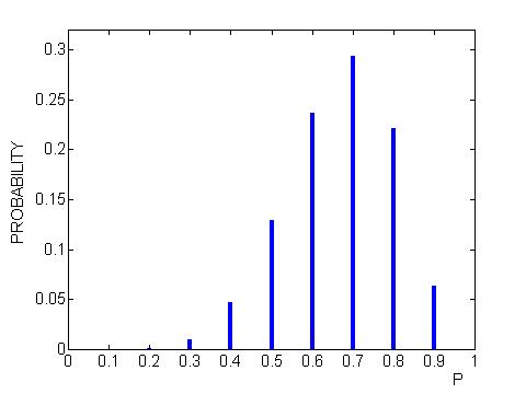
We illustrate computing the posterior probabilities for the proportion p using the Minitab macro p_disc. To use this program, one places the values of p into a single column in the Minitab data table and the corresponding prior probabilities in a different column. In the output below, these columns are named 'p' and 'prior'. The computation of the posterior is accomplished by the Minitab command (typed in the Session Window)
MTB > %p_disc 'p' 'prior' 7 3The Minitab output from this command is a Bayes' Table, showing values of p, the prior probabilities, the likelihood, the products, and the posterior probabilities.
PRIOR AND POSTERIOR DENSITIES OF P:

 Row      P       PRIOR       LIKE   PRODUCT      POSTR

   1    0.0   0.0909091          0       0.0   0.000000
   2    0.1   0.0909091         33       3.0   0.000010
   3    0.2   0.0909091       2947     267.9   0.000864
   4    0.3   0.0909091      33736    3066.9   0.009892
   5    0.4   0.0909091     159156   14468.7   0.046668
   6    0.5   0.0909091     439188   39926.1   0.128779
   7    0.6   0.0909091     805728   73248.0   0.236256
   8    0.7   0.0909091    1000000   90909.1   0.293220
   9    0.8   0.0909091     754518   68592.6   0.221240
  10    0.9   0.0909091     215104   19554.9   0.063073
  11    1.0   0.0909091          0       0.0   0.000000
A line graph of the posterior probabilities of p is shown below.
Using this posterior probability distribution, we can answer different inferential questions.
What's my best guess at the relative abilities of Agassi
and Becker?
We measure the relative abilities of the two players by p, the proportion of
times Agassi would win if the two players played an infinite number of
matches. One best guess of p is the value which is assigned the
largest probability (the mode). Looking at the posterior probability
table, we see that p = .7 has the largest probability -- so p = .7 would be
our best guess.
Can I construct an interval of values where I am
confident contains the unknown value of p?
Here we find a set of values of proportion values p which contains a
high, say 90%, of the posterior probability distribution. A simple way
of finding this interval is to arrange the values of p from most likely to
least likely, and then put values of p into the interval until the
cumulative probability of the set exceeds .9.
Below I have sorted the proportion values from most likely to least
likely. Looking at the "cum prob" column, we see that the
probability that p is in the set {.7, .6, .8, .5, .9} is .9426. So
this set is a 90% probability interval for p.
| p | prob | cum prob |
| 0.7 | 0.2932 | 0.2932 |
| 0.6 | 0.2363 | 0.5295 |
| 0.8 | 0.2212 | 0.7507 |
| 0.5 | 0.1288 | 0.8795 |
| 0.9 | 0.0631 | 0.9426 |
| 0.4 | 0.0467 | 0.9892 |
| 0.3 | 0.0099 | 0.9991 |
| 0.2 | 0.0009 | 1.0000 |
| 0.1 | 0.0000 | 1.0000 |
| 0 | 0.0000 | 1.0000 |
| 1 | 0.0000 | 1.0000 |
What is the probability that Agassi is the better
player?
Remember that p is the proportion of matches Agassi would win against
Becker if they played a large number of matches. To say that Agassi is
the better player means that p is larger than .5. From the posterior
probability table, we compute
Prob(p > .5) = Prob(p = .6, .7, .8, .9, 1) = .236 + .293 + .221 + .063 =
.813
Since this probability (.813) is moderately large, we have some confidence
that Agassi is the superior player.
Page Author: Jim Albert (c)
albert@math.bgsu.edu
Document: http://math-80.bgsu.edu/nsf_web/main.htm/primer/topic16.htm
Last Modified: October 17, 2000