Introduction
As in the previous topic, we are interested in learning about a population proportion p. What is different here is how we represent prior beliefs about the proportion. In Topic 16, we specified a discrete prior by first specifying a set of possible values of p, and then specifying probabilities to these values. Here we assume that the proportion p is continuous-valued on the interval (0, 1), and then specify a prior distribution by means of a curve defined over this interval. We will see that the calculation of posterior probabilities for p is straightforward when p has a prior density that is a beta curve.
Continuous Models for a Proportion
When we used a discrete prior for the proportion p in Topic 16, we assumed that p could take on a specific set of values like 0, .1, .2, ..., 1. But this is a bit restrictive and unrealistic. Why can't p take on other values, such as .15, or .143, or even .143122? Generally, since the proportion is really continuous-valued and possibly could be any number between 0 and 1, it makes sense to specify a prior probability distribution for p on the interval (0, 1).
How do we specify probabilities for a continuous-valued unknown quantity like p?
Uniform Curves
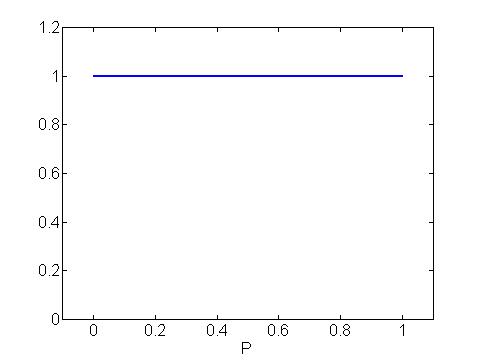
First suppose that we have no idea about the location of the proportion p, and so p is equally likely to be any value between 0 and 1. If p only took on the discrete set of values 0, .1, ..., .9, 1, then we would assign a probability of 1/11 to each of the 11 possible values. If we had a finer set of values, say p = 0, .01, .02, ..., .99, 1, there are 101 possible values and, if we knew nothing about this proportion, a probability of 1/101 would be assigned to each value. If we let p take on a large number of values, then the picture of the probability distribution would resemble the uniform curve shown below. A curve like this one is how we represent beliefs about a continuous-valued parameter like p.
Finding Probabilities
When the proportion p is continuous, we can't sum probabilities like we did in the discrete case. There is an infinite number of possible values, and if we summed all the values of p, it would be impossible to get a probability which is no larger than 1. In this continuous case, we find probabilities by computing areas under the curve.
It is convenient to introduce the notion of areas as probabilities in the case where p has a uniform curve. Suppose that we are interested in the probability
P(.3 < p < .6).
We find this probability by computing the area under the uniform curve between the values .3 and .6. This area is shaded as a red rectangle in the graph below. By using the AREA = BASE x HEIGHT formula to find the area of this rectangle, it is easy to see that the probability of interest is equal to .3.

By the way, notice that P(0 < p < 1) is represented by the area under the entire curve between 0 and 1 which is equal to 1. This is true for all probability curves -- the total area under the curve is equal to 1. This result is analogous to the result that the sum of probabilities of a discrete distribution is equal to 1.
Beta Curves
We use a uniform curve as our prior when we have little knowledge, before sampling, about the location of the proportion p. But what if we do have information about p? Then we use a member of a special class of curves, the beta curves, to represent our knowledge about the proportion.
The beta prior curve has the basic form
![]()
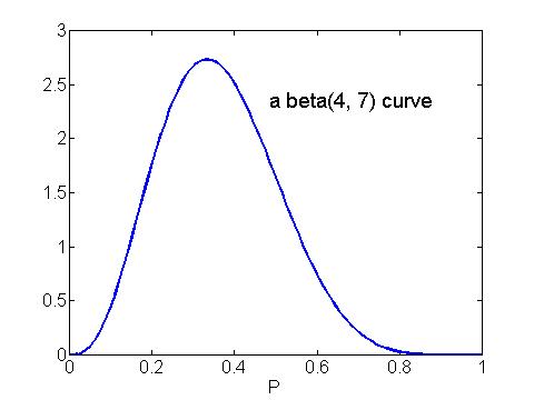
The shape and location of this curve are determined by the two beta numbers a and b. The beta curve with numbers a = 4 and b = 7 is shown below -- we call this a beta(4, 7) curve. We will shortly discuss how a person chooses the values of the beta numbers to reflect his or her information about p.
Beta Probabilities
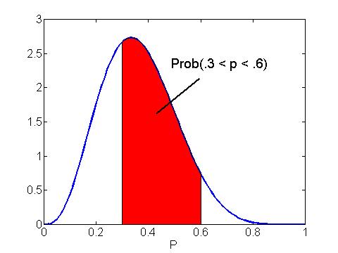
If we represent our beliefs about the proportion p in terms of a beta curve, then we compute probabilities about p, say Prob(.3 < p < .6), by computing areas under the beta curve. In the figure below, we shade the region under the beta(4, 7) curve between .3 and .6 which corresponds to the probability of interest. We compute this shaded area using special Minitab commands or a javascript program that is available with the book. Using these programs we find that
Prob(.3 < p < .6)= .5948.
So the chance that the population proportion is between .3 and .6 is approximately .59.
Beta Percentiles
We are also interested in computing percentiles for a beta curve. The 30th percentile, p30, is the value of the proportion such that the probability that the proportion is less than that value is .3. That is,
P(p < p30) = .3 .
The 30th percentile of a beta(4, 7) curve is illustrated in the figure below. The red region is the "less than" area that we wish to be equal to .3.

We find a percentile of a beta curve by using Minitab or a special javascript program. To use these problems, one inputs the numbers a and b of the beta curve and the area to the left, and the program gives the appropriate beta percentile.
Probability Interval
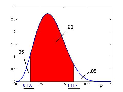
One is often interested in computing a probability interval for p. This is an interval that contains the proportion with a prescribed probability. One can find a probability interval by computing two percentiles for the beta curve. Suppose that our prior curve is beta(4, 7) and we want a 90% probability interval, that is, an interval which contains 90% of the total probability under the curve. A convenient way of finding this interval is the so-called "equal-tails" interval where half of the remaining probability (.05) is to the left of the interval and half of the probability (.05) is to the right. Then the percentiles (p05, p95) will be our 90% probability interval. The figure below shows the shaded 90% probability and the "equal-tails" interval (.150, .607) that is found using a program (such as Minitab or the javascript program) that computes percentiles of the beta curve
Constructing a Beta Curve
The beta family of curves is a flexible collection of curves to represent a person's knowledge about a population proportion. To use this family, the person needs to specify the beta numbers a and b. In the book, we present a simple method of obtaining values of a and b which approximately represents a person's information about the parameter.
One assesses values of the beta numbers a and b by
For example, suppose that you are interested in learning about the proportion of potential voters p who are supportive of the Republican candidate. Before sampling, you think that
So in this example, g would be .4 and n would be 20. If you were more sure of your belief, then you would use a larger value of n. On the other hand, if you were very unsure about your guess that p is equal to .4, then you would use a small value of n.
Once you obtain values of g and n, then the beta numbers are given by
a = n g, b = n (1 - g).
In our example, since g = .4 and n = 20, we have
a = 20 (.4) = 8, b = 20 (.6) = 12 .
You would use a beta(8, 12) curve to model your beliefs about the proportion of voters for the Republican.
Generally, it is difficult to specify g and n since one has not had much practice doing it. After one obtains the beta numbers a and b using the above method, it is recommended to plot the beta(a, b) curve and compute a few percentiles or probabilities under the chosen curve. If the beta curve doesn't appear to match one prior beliefs, then one can modify the values of g and n to get a better approximation to one's information. By use of several iterations of this trial and error approach, one can obtain a beta curve that seems to reflect one's knowledge about the proportion p.
Inference Using a Beta Curve
After one constructs a beta curve to model one's prior information about the proportion p, data is collected. Suppose a random sample is taken from the population and s successes and f failures are observed. From Topic 16, we know that the likelihood of this data is given by
![]()
The prior curve, from above, has the form
![]()
By Bayes' rule, the posterior curve for p is obtained by multiplying the prior and likelihood:
![]()
![]()
![]()
We recognize the posterior curve as a beta curve with numbers a+s and b+f; that is, a beta(a+s, b+f) curve.
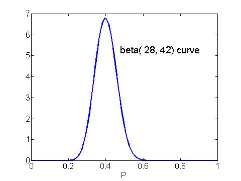
Let's return to our voting example in which the proportion p of voters in favor of the Republican candidate has a beta(8, 12) prior curve. Suppose a random sample of 50 voters is taken and 20 are in favor of the Republican; here s = 20 and f = 30. The posterior curve is beta with numbers
a + s = 8 + 20 = 28, b + f = 12 + 30 = 42 .
This curve is pictured below.
Inference about the proportion p is done by computing appropriate summaries of this beta curve.
To illustrate, suppose one is interested in estimating p by a 95% probability interval. We find the 2.5th and 97.5th perc entiles of the beta(28, 42) curve to be
(p2.5, p97.5) = (.2891, .5163).
This interval contains 95% of the area under the beta curve and so is a 95% probability interval for p. Note that this interval contains values on both sides of .5. Thus we are not confident that the proportion of voters favoring the Republican candidate is smaller than .5.
Inference Using a Uniform Curve
Sometimes the user may have little prior knowledge about the location of the population proportion p. Then it is reasonable to use a prior curve for p which reflects vague, or imprecise knowledge about this proportion. One prior that reflects this lack of knowledge is the uniform curve
![]()
This can be seen to be a special case of a beta curve with a = 1 and b = 1. Applying our previous result with a beta prior, if we observe s successes and f failures in our sample, the posterior density for p will be beta with numbers s + 1 and f + 1.
Returning to our voting example, suppose that a person has little knowledge about the proportion of voters in favor of the Republican candidate and assigns a uniform prior curve. Then, if we observe 20 voters in favor and 30 voters not in favor, then the posterior curve for p will be beta(1 + 20, 1 + 30) = beta(21, 31).
We find the 2.5th and 97.5% percentiles of a beta(21, 31) curve to be .2758 and .5389, respectively. So a 95% probability interval for p is given by (.2758, .5389). Note that there are differences between the probability intervals using the beta(8, 12) prior curve and the uniform prior curve. This difference in intervals is due to the different information in the two prior curves.
Page Author: Jim Albert (c)
albert@math.bgsu.edu
Document: http://math-80.bgsu.edu/nsf_web/main.htm/primer/topic17.htm
Last Modified: October 17, 2000