Introduction
This topic introduces Bayesian inference for a population mean. We have a population of continuous measurements and we are interested in learning about the mean M of the populations. As a simple example (Berry, 1996), suppose that you are measuring your weight (in pounds) on a scale. From experience, you know that the weight readings from the scale are variable and you imagine a population of measurements obtained by weighing yourself many times. You wish to learn about the mean M of this population of weight measurements.
A Normal Curve Model
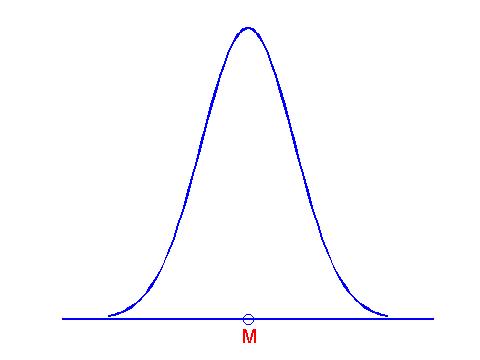
How do we define a model for measurements? First, we assume that the distribution of measurements in the population can be described by a normal curve. This normal curve is described by two numbers -- a mean M and a standard deviation h. In this topic, we assume that we know the value of the population standard deviation h, and focus on learning about the population mean M.
This situation is conceptually more difficult than learning about a proportion. In that case, a model was simply described by a number p that represented the proportion of successes in the population. Here a model is not a single number, but rather a distribution of measurements that is centered about the unknown mean value M. The figure below shows this normal curve model.
Formula for a Normal Curve
In the following, we will need to know the formula for the normal curve that describes the population of measurements. If x denotes a measurement, then the normal curve is given by
![]()
where z is the standardized score obtained by subtracting the mean M and dividing by the standard deviation h

Collection of Normal Models
To learn about the population mean M, we use the same discrete model approach that we followed in Topic 16 for a population proportion. First, we think of several plausible values for the population mean, and then assign probabilities to the different values of M that reflect our knowledge about likely or unlikely values.
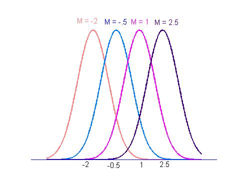
Suppose that we know the standard deviation of the population is h = 1, and we think that the population mean values M = -2, -.5, 1, 2.5 are all possible. The four population measurement models are graphed in the figure below. Note that all of the models have the same shape (since all have the same standard deviation). The only difference is in the location of the four curves.
In our weighing example, M is the mean of an infinite collection of measurements taken from my scale. What are plausible values for M? If I assume that the average measurement M from the scale represents my true weight, then I would list several values for my true weight that are displayed in the table below.
| M (pounds) |
| 140 |
| 142 |
| 144 |
| 146 |
| 148 |
| 150 |
| 152 |
| 154 |
| 156 |
Prior
After a list of plausible values for M is made, probabilities are assigned; that reflect my beliefs about the likelihood of the different values.; In this case, suppose that I think that each of the nine values listed above are equally plausible, resulting in the following assignment of prior probabilities.
| M(pounds) | PRIOR |
| 140 | 1/9 |
| 142 | 1/9 |
| 144 | 1/9 |
| 146 | 1/9 |
| 148 | 1/9 |
| 150 | 1/9 |
| 152 | 1/9 |
| 154 | 1/9 |
| 156 | 1/9 |
Computing Posterior Probabilities Using One Observation
Suppose that I weigh myself one time and the reading is 147 pounds. What have I learned about my true weight?
We compute the new or posterior probabilities for M by means of Bayes' rule.
Likelihoods. For each model, we compute the likelihood which is the probability of our observed data. Suppose that our data result is denoted by x. Then the likelihood of the model M is given by
![]()
where z is the standardized score
In this example, our observed measurement is x = 147. Suppose that we know (from previous experience working with scales) that the standard deviation of the population of measurements is h = 2. Then the likelihood would have the above form, where the standardized score is
Bayes' rule. Once the likelihoods are defined, then posterior probabilities for the population mean M are defined using the familiar "multiply, sum, divide" recipe that we used to compute posterior probabilities in Topic 16 for a population proportion. The calculations are shown in the following Bayes' table.
 M   PRIOR     Z     LIKELIHOOD PRODUCT	 POSTERIOR
--------------------------------------------------
140  .1111  -3.5000    0.0022    0.0002    0.0009
142  .1111  -2.5000    0.0439    0.0049    0.0175
144  .1111  -1.5000    0.3247    0.0361    0.1295
146  .1111  -0.5000    0.8825    0.0981    0.3521
148  .1111   0.5000    0.8825    0.0981    0.3521
150  .1111   1.5000    0.3247    0.0361    0.1295
152  .1111   2.5000    0.0439    0.0049    0.0175
154  .1111   3.5000    0.0022    0.0002    0.0009
156  .1111   4.5000    0.0000    0.0000    0.0000
What have I learned about my true weight? Initially I thought that each of the nine possible means 140, ..., 156 had the same probability. Now, after observing my single measurement, I note that the two values M = 146 and M = 148 have the largest probabilities of .3521. To get some idea of the uncertainty in my knowledge about the mean, we can find a set of values which contains M with a high probability. Looking at the posterior probability table, we see that
Prob(M = 144, 146, 148, 150) = .1295 + .3521 + .3521 + .1295 = .9632 .
So the set {144, 146, 148, 150} is a 96.32% probability interval for the mean M of the population of weight measurements.
Computing Posterior Probabilities Using a Sample of Observations
Actually we didn't learn about the mean M of measurements above, since we took only a single reading. Suppose instead that we can take a sample of n independent measurements x1, ..., xn. How do we perform inference about M in this situation?
The only change is how we compute the likelihoods. In the case where we have independent observations, then the likelihood for M is found by multiplying the probabilities of the individual data values.
![]()
where z1, ... , zn are the standardized scores for the n observations.
z1 = (x1 - M)/h, ..., zn = (xn - M)/h
It turns that one can show that this product is equivalent to
![]()
where zm is the standardized score of the sample mean
To compute the posterior probabilities for the values of M, we follow the same Bayes' rule recipe as we did in the single observation case. To illustrate, suppose that I take five measurements from my scale:
147, 146, 150, 147, 145
Here we have taken n = 5 measurements and

To compute the likelihoods, we first compute the standardized scores
for each possible value of M, and then LIKELIHOOD = exp(-zm2/2). The table following displays the posterior probabilities after observing these five weighings.
M   PRIOR LIKELIHOOD POSTERIOR
----------------------------
140  .1111   0.0000  0.0000
142  .1111   0.0000  0.0000
144  .1111   0.0036  0.0033
146  .1111   0.5353  0.4967
148  .1111   0.5353  0.4967
150  .1111   0.0036  0.0033
152  .1111   0.0000  0.0000
154  .1111   0.0000  0.0000
156  .1111   0.0000  0.0000
Note that we have learned more about the mean M from this sample of size 5 than we did from a single weighing. The probability that M is 146 or 148 is .4967 + .4967 = .9934 and so it is extremely unlikely that my true weight is smaller than 146 or larger than 148.
Page Author: Jim Albert (c);
albert@math.bgsu.edu;
Document: http://math-80.bgsu.edu/nsf_web/main.htm/primer/topic18.htm;
Last Modified: October 17, 2000