
Introduction
This topic is a continuation of the discussion in Topic 18 about learning about a population mean. We have a population of measurements that we assume is normally distributed with unknown mean M and known standard deviation h. In our example, suppose you are interested in your true weight M and you take repeated weighings from a scale. The distribution of weighings is assumed normal-shape with mean M. You wish to learn about your true weight from the measurements that are taken.
A Continuous Set of Normal Curve Models
In Topic 18, prior opinion about the population mean was represented by means of a discrete distribution. A set of plausible values for M was found, and probabilities were assigned to the values of M in the set that corresponded to your prior beliefs about the relative likelihoods of the values. This process is a bit unrealistic since the population mean M can really take on a continuum of values. For example, you might think that your true weight M is 175, 176, or 177. But certainly your true weight could be 175.5 or 176.12 or even 175.12456. In this topic, we assume that M is a continuous unknown quantity, so actually there would be an infinite number of possible normal curve models for the population of measurements. When M is continuous, we model our prior information using a probability curve.
Probability Curve
When one has a continuous unknown quantity such as M, we represent probabilities using a smooth curve called a probability curve. A normal probability curve is displayed below. It is instructive to consider this special probability curve, since inferences about the population mean will be based on the normal curve.
There are several properties that define a probability curve. First, the curve must lie on or above x-axis; that is, the curve only takes on non-negative values. Second, the total area under the curve is equal to 1; this property is similar to the property for discrete distributions that the sum of the probabilities is equal to 1.
Finding Probabilities
We find probabilities by computing areas under the probability curve. To illustrate, the above curve is a normal curve with mean 100 and standard deviation 15. This curve represents my beliefs about the IQ test score X for an "average" individual. What is the probability that the individual obtains a test score less than 90? We find this probability by computing the area over values of X smaller than 90 .
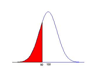
This type of "less than" area is conveniently computed by use of a table or a computer program. In the Javascript program [name], we input the mean (100) and standard deviation (15) of the normal curve, and the value of X (90) of interest. The program gives
Prob(X smaller than 90) = .2524 .
Two other types of probabilities that we might be interested in are "greater than" probabilities, and probabilities "between two values". Suppose, for example, we wish to find the probability that the test score exceeds 120.
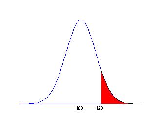
We find this by first computing the probability that the score is less than 120.
Prob(X less than 120) = .9087 .
Since the entire area under the normal curve is equal to 1, we find the probability of interest by subtracting the "less than" probability from 1.
Prob(X greater than 120) = 1 - Prob(X less than 120) = 1
- .9087
= .0913
Next, suppose we wish to find the probability that the test score is between 90 and 105, as shown in the figure below.
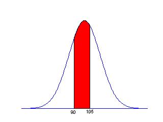
We find this area by subtracting two areas -- we subtract the area to the left of 90 from the area to the left of 105.
P(X is between 90 and 105) = P(X less than 105) - P(X less than 90)
= .6307 - .2524 = .3783 .
Finding Percentiles
It is also of interest to find percentiles of a probability curve. These are values that contain specific probabilities or areas under the curve. The 20th percentile is the value of the variable X such that 20% of the probability is less than that value. For example, suppose we wish to find the 20th percentile of the distribution of IQ scores. This percentile is the particular test score such that the area to the left of the score is equal to .2. (See the figure below.)
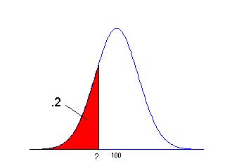
We compute a percentile by using a specific program such as the Javascript program [name] supplied with the book. To use this program, we input the mean (100) and standard deviation (15) of the normal curve and the area to the left (.2) -- the program gives
20th percentile of test scores = 87.41
We can say 20% of the IQ scores were smaller than 87.41 and so 80% of the scores were greater than 87.41.
A Uniform Prior
We use a probability curve to represent our knowledge about a continuous-valued parameter such as a population mean. Suppose you have little knowledge about the value of M. In this situation, your prior beliefs can be represented by a uniform or flat curve.
This prior curve isn't actually a honest probability curve, since the total area under the curve is infinite. But it is reasonable approximation to one's prior beliefs when you have little information about M. Also, as we will shortly see, although the prior curve is not a true probability curve, the posterior curve will be a legitimate probability distribution.
Inference About a Mean Using a Uniform Prior
Suppose we take a sample of n measurements x1, ..., xn and we represent our prior beliefs about the population mean M are represented by a uniform curve. By Bayes' rule, the posterior curve for M is found by the basic recipe
POSTERIOR = LIKELIHOOD x PRIOR,
where LIKELIHOOD is the probability of the observed measurements given a value of the population mean. In Topic 18, we showed that one can express the likelihood as
![]()
where zm is the standardized score of the sample mean
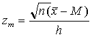 .
.
Since
the prior curve is uniform, the posterior curve is equivalent to the likelihood
viewed as a function of the population mean M. This is recognized as
a normal curve with mean
![]() and standard deviation h/sqrt(n).
and standard deviation h/sqrt(n).
In our example, suppose we take five measurements from the scale, obtaining the weights (in pounds)
147, 146, 150, 147, 145
Here we have taken n = 5 measurements and

Suppose also that we know the standard deviation of the population is equal to h = 2. Then the posterior curve for your true weight M will be normal with mean 147 and standard deviation 2/sqrt(5) = .894. This posterior curve is shown below.
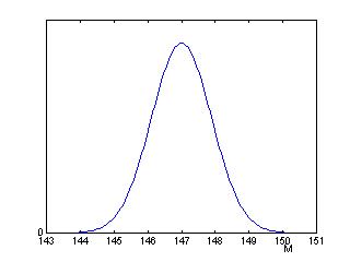
All inferences about the population mean are based on this probability curve. We illustrate several types of inferences here.
What is the probability that your true weight is larger than 150?
We simply compute P(M > 150). Using the normal probability program, we find that P(M < 150) = .9994. So the probability that your true weight is larger than 150 is equal to 1 - .9994 = .0006.
Can I find an interval which contains my true weight with probability .9?
To find a 90% probability interval for M, we find the 5th and 95th percentiles of the normal (147, .894) curve. Using the normal percentile program, we find the two percentiles to be 145.53 and 148.47. So (145.53, 148.47) is a 90% probability interval for your true weight M.
What if the Standard Deviation is Unknown?
All of the computations above implicitly assume that we know the population standard deviation h exactly. Usually we don't know this population standard deviation, but we can compute the standard deviation s from the sample. In this case where h is unknown, we substitute the value

for h in the above formula. Note that we are substituting a value for h that is slightly larger than the sample standard deviation s. When we find a probability interval for M, we will obtain a longer interval then the interval found when h is known. Since we don't know h, there is some uncertainty in using an estimate (s) instead of h, and we pay for this uncertainty by means of a longer interval for the population mean M.
A Normal Prior
Up to this point, we have assumed that you have little prior information about the location of the population mean M, and have used a uniform curve to represent your vague knowledge about M. But what if you have some knowledge, before you look at any data, about plausible values for M? In that case, you would want to use a proper probability curve instead of the uniform curve to represent your knowledge. A convenient choice for this curve is a normal curve with mean m0 and standard deviation h0.
This curve is centered about the value m0. This means that you think that the most likely value for the population mean M is m0. The sureness of this belief is measured by the standard deviation h0. If you are really sure that the population mean M is close to m0, a small value of h0 would be chosen, and the probability curve would be concentrated about m0. In contrast, if you chose the standard deviation h0 to be a large value, this indicates that you are unsure about the value of the population mean M and the curve will be very spread out about the mean value m0.
Assessing a Normal Prior
Generally, it is difficult to specify a normal probability curve to reflect one's prior information about a population mean M. This topic suggests one simple method of determining the values of the prior mean m0 and the prior standard deviation h0. This method essentially matches one's prior beliefs about two percentiles of the probability curve of M to the values of m0 and h0.
Suppose that you can make intelligent guesses at
the median of M (call it m0)
the pth percentile mp
Then a normal curve with mean m0 and standard deviation h0, where the standard deviation is given by the formula
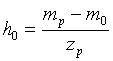
will match this information. In the formula, zp denotes the value of the pth percentile of a normal curve with mean 0 and standard deviation 1.
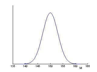
Let's illustrate this procedure for the problem of learning about your true weight M. First you make an intelligent guess at your weight -- after some thought you decide that m0 = 150 pounds. Next, you guess at the 90th percentile at your true weight. This is a weight value that you are 90% confident that your true weight M is smaller than that value. After some reflection, you decide that you are pretty confident that your weight is smaller than 155 pounds. So m90 = 155.
To use the formula, we first find the 90th percentile of a normal curve to be 1.645. Then we compute
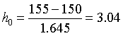
So a normal curve with mean 150 and standard deviation 3.04 approximately matches your prior information about your true mean M. We plot this curve below.
Inference About a Mean Using a Normal Prior
In the situation where our prior beliefs about the population mean M are described by a normal curve, we use Bayes' rule to make inferences about M after data are observed. We use the basic recipe
POSTERIOR = LIKELIHOOD x PRIOR,
where LIKELIHOOD is shown above and PRIOR represents the normal probability curve with mean m0 and standard deviation h0. When one does this multiplication and simplifies the expression, it can be shown that the posterior curve will also have a normal form with mean
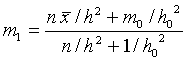
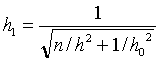
and standard deviation
The table below gives a convenient way of performing the calculations of the mean and standard deviation of the posterior curve for M. In doing this, it is helpful to define the precision c which is the reciprocal of the square of the standard deviation.
c = 1 / h2.
We compute the posterior mean and standard deviation for M by completing the table as follows.
We first place the mean and the standard deviation of the
normal prior in the "Mean" and "Standard Deviation"
columns in the "Prior" row of the table. Likewise, we place
the sample mean xbar and the data standard deviation h/sqrt(n) in the
"Data" row of the table.
Next, we find the precisions of the Prior and the Data using
the formula c = 1/h2.
We find the precision of the Posterior, c1, by
adding the precisions of the Prior to the precision of the Data.
We compute the standard deviation of the precision by using
the formula h1= 1/sqrt(c1).
Last, we find the posterior mean using the formula m1 = (c0 m0 + cD xbar)/c1
| Mean | Standard Deviation | Precision | |
| Prior | m0 | h0 | c0=1/h02 |
| Data |
|
|
cD=n/h2 |
| Posterior | m1 |
|
c1 = c0 + cD |
We illustrate these calculations for the weighing example where your prior beliefs about your true weight M are described by a normal curve with mean 150 and standard deviation 3.04. We put these values in the Prior row of the table. Likewise, we place the observed sample mean 147 and the corresponding data standard deviation h/sqrt(n) = .894 in the Data row. Then
We compute the precisions of the prior and data from the
given standard deviations. By adding the prior and data precisions we
obtain the precision of the posterior curve:
Posterior Precision = .108 + 1.251 = 1.359
We compute the standard deviation of the posterior curve
from the posterior precision:
Posterior Standard Deviation = 1/sqrt(1.359) = .858
Last, we compute the mean of the posterior as
Posterior Mean = [ (.108) (150) + (1.251) (147) ]/1.359 = 147.2
| Mean | Standard Deviation | Precision | |
| Prior | 150 | 3.04 | 0.108 |
| Data | 147 | .894 | 1.251 |
| Posterior | 147.2 | .858 | 1.359 |
The posterior curve for M combines the information from two sources -- the prior and the data. Initially, before any data were collected, you believed that your true weight M was in the vicinity of 150 pounds. This belief is represented by the red prior curve in the figure below. You then took five measurements from the scale -- the data tells you that your true weight M is in the neighborhood of 147 pounds. The likelihood function that reflects the information from the data is represented by the black curve. The posterior curve, represented in the figure by the blue curve, lies between the prior curve and the likelihood function. Here there is much more information provided by the data than by your prior belief (you weren't really that sure about your true weight), and so the posterior curve falls much closer to the likelihood than your prior.

Page Author: Jim Albert (c)
albert@math.bgsu.edu
Document: http://math-80.bgsu.edu/nsf_web/main.htm/primer/topic19.htm
Last Modified: October 17, 2000