A Brief Tutorial on Bayesian Thinking

Example:  learning about a proportion

We first discuss the similarities and differences between classical and Bayesian methods for a problem of learning about a population proportion.  For a particular Big Ten university, we are interested in estimating the proportion p of athletes who graduate within six years.  For a particular year, forty-five of seventy-four athletes admitted to the university graduate.  Assuming that this sample is representative of athletes admitted during other years, what have we learned about the proportion of all athletes who will graduate within six years?  Specifically, we will consider two types of inferences. 

• We wish to construct an interval that we are pretty confident contains the unknown value of p.  

• Suppose that the university would like to state that over half of its athletes graduate on time --- that is, p is larger than .5.  Can the university make this statement with some confidence?

The classical approach

The classical 95% interval estimate for the proportion $p$ for a large sample is given by

where denotes the sample proportion of athletes who graduate within six years, and n is the size of the sample.  In this example = 45/74 = .608$ and n = 74$ and, by substitution in the above formula, one obtains the interval (.497, .719).

If the university wishes to show that the proportion p is larger than one half, then the classical approach would test the null hypothesis H:  p <= .5 against the alternative hypothesis K: p > .5.  One decides between the hypotheses on the basis of a p-value.  In this example,  one finds the probability that the sample proportion , in repeated sampling, is equal to or greater than the observed value = .608 when p = .5.  Using binomial tables, one finds that the p-value is equal to .0403.  If the level of significance is .05, one concludes that there is sufficient evidence that the proportion of athletes who graduate exceeds one-half.

The Bayesian approach

A different way of thinking about probability

The Bayesian approach to learning is based on the subjective interpretation of probability.   The value of the proportion p is unknown, and a person expresses his or  her opinion about the uncertainty in the proportion by means of a probability distribution placed on a set of possible values of p. 

Prior and posterior probabilities

The prior distribution is the probability distribution that the person has before observing data.  After observing data, the person changes his or her opinion about the value of the proportion.  The new probability distribution, the posterior distribution, is computed using Bayes' rule.  All of the person's knowledge about the proportion is contained in the posterior distribution, and statistical inferences are made by summarizing this distribution.

Revisit the example

Let us reanalyze our example from a Bayesian perspective.  Suppose that little is known about the location of the proportion p.  We construct a prior distribution for this proportion that reflects this belief.   Suppose that p could conceivably be any one of the ninety-nine values .01, .02, ..., .99.   If we know very little about the proportion, we may think that these values for p are equally likely, and so we assign to each value the probability 1/99.

After observing the graduation results, we update our probability distribution for using Bayes' rule.   Let's illustrate this calculation for the single value p = .5.  By Bayes' rule

Prob(p = .5 given data) is proportional to P(p = .5) x P(data given p = .5).

Here

• P(p=.5) is our prior probability of 1/99
  

• P(data given p = .5) is the probability of getting our data result (45 graduate out of 74 athletes) if the true proportion is indeed equal to .5.  By the binomial formula, this probability is equal to
  
  

So, by Bayes' rule',

Prob(p = .5 given data) is proportional to

In general, the posterior probability that the proportion p is exactly equal to p0 is proportional to

    Prob(p =p0 given data) is proportional to

Interpreting the posterior distribution

If we perform the above calculation for each of the 99 possible values of p, and then normalize the probabilities so that they sum to one, we obtain the following posterior probability distribution.  We represent it by a table and by a graph.

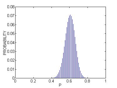
This probability distribution represents our current opinion about the graduating proportion of the football players.

Best guess at the proportion

We can estimate the unknown proportion p by some average value of the above posterior probability distribution.  One reasonable estimate of p is the mode, or the most likely value.  From the table above, we see that the mode is equal to .61, although the chance that p is exactly equal to .61 is only about 7%.

A 95% Bayesian probability interval

A 95% probability interval for the proportion is found by finding a collection of values of p with a probability content that is approximately .95.

Here we obtain the  set {.50, .51, ..., .71}, which is approximately equal to the 95% confidence interval found using the classical method. 

Interpretation of the interval

Although the classical and Bayesian intervals agree, the interpretations of the two intervals are different.  The probability of the proportion p falling in the Bayesian interval [.50, .71] for this data set is actually 95%.  In contrast, from a classical perspective, one is not confident that the interval (.497, .719) contains p.  The classical statistician is confident about the procedure --- if this 95% interval is computed for repeated sampling, then we are confident that approximately 95% of the intervals will contain the proportion value. 

A Bayesian test

Next, consider the question whether over half of the athletes graduate within six years.  From a Bayesian viewpoint, the plausibility of the hypothesis H: p <= .5 is found by computing its posterior probability.  From the set of posterior probabilities, one finds that the probability the proportion value is less than or equal to  one-half is .032.  This probability is small, so we would conclude that there is good evidence that over half of the athletes graduate on time.  Note that the posterior probability of the hypothesis H is approximately equal to the classical p-value.

For this example, the classical procedures gave similar answers to the Bayesian procedures when a weak or noninformative prior distribution was used.  However, there are important distinctions between the two sets of procedures.  One difference is the interpretation.  The Bayesian computes probabilities about the unknown proportion p conditional on the sample that is observed.  In contrast, the classical statistician has no confidence that he of she is correct for this data set.  The confidence comes from repeating this inferential process for many data sets.

What's attractive about Bayes' thinking?

The Bayesian mode of inference has a number of desirable features.

Inferential statements are easy to understand

One attractive feature is that inferential statements about a parameter are easy to communicate.  It is natural to talk about the probability that p falls in an interval or the probability that a hypothesis is true. 

One recipe

A second nice feature is that a single recipe, Bayes' rule, is used for updating one's probabilities about a parameter.  This rule can be used for small or large sample sizes. 

Mechanism for using subjective beliefs in a problem

Bayesian methods allow a person to use his or her subjective beliefs about the location of the parameter in the inference problem.  In our example, one may have some opinions about graduating rates of athletes based on data from other universities, and a prior probability distribution for p can be constructed to reflect this knowledge.  Bayes' rule provides a useful mechanism for combining this prior knowledge about the graduation rates with information contained in the sample.