Chapter 6 Joint Probability Distributions
6.1 Introduction
In Chapters 4 and 5, the focus was on probability distributions for a single random variable. For example, in Chapter 4, the number of successes in a Binomial experiment was explored and in Chapter 5, several popular distributions for a continuous random variable were considered. In addition, in introducing the Central Limit Theorem, the approximate distribution of a sample mean \(\bar X\) was described when a sample of independent observations \(X_1, ..., X_n\) is taken from a common distribution.
In this chapter, examples of the general situation will be described where several random variables, e.g. \(X\) and \(Y\), are observed. The joint probability mass function (discrete case) or the joint density (continuous case) are used to compute probabilities involving \(X\) and \(Y\).
6.2 Joint Probability Mass Function: Sampling From a Box
To begin the discussion of two random variables, we start with a familiar example. Suppose one has a box of ten balls – four are white, three are red, and three are black. One selects five balls out of the box without replacement and counts the number of white and red balls in the sample. What is the probability one observes two white and two red balls in the sample?
This probability can be found using ideas from previous chapters.
First, one thinks the total number of ways of selecting five balls with replacement from a box of ten balls. One assumes the balls are distinct and one does not care about the order that one selects the balls, so the total number of outcomes is \[ N = {10 \choose 5} = 252. \]
Next, one thinks about the number of ways of selecting two white and two red balls. One does this in steps – first select the white balls, then select the red balls, and then select the one remaining black ball. Note that five balls are selected, so exactly one of the balls must be black. Since the box has four white balls, the number of ways of choose two white is \({4 \choose 2} = 6\). Of the three red balls, one wants to choose two – the number of ways of doing that is \({3 \choose 2} = 3\). Last, the number of ways of choosing the remaining one black ball is \({3 \choose 1} = 3.\) So the total number of ways of choosing two white, two red, and one black ball is the product \[ {4 \choose 2} \times {3 \choose 2} \times {3 \choose 1} = 6 \times 3 \times 3 = 54. \]
Each one of the \({10 \choose 5} = 252\) possible outcomes of five balls is equally likely to be chosen. Of these outcomes, 54 resulted in two white and two red balls, so the probability of choosing two white and two red balls is \[ P({\rm 2 \, white \, and \, 2 \, red}) = \frac{54}{252}. \]
Here the probability of choosing a specific number of white and red balls has been found. To do this calculation for other outcomes, it is convenient to define two random variables
\(X\) = number of red balls selected, \(Y\) = number of white balls selected.
Based on what was found, \[ P(X = 2, Y = 2) = \frac{54}{252}. \]
Joint probability mass function
Suppose this calculation is done for every possible pair of values of \(X\) and \(Y\). The table of probabilities is given in Table 6.1.
Table 6.1. Joint pdf for (\(X, Y\)) for balls in box example.
| \(X\) = # of Red | 0 | 1 | 2 | 3 | 4 |
| 0 | 0 | 0 | 6/252 | 12/252 | 3/252 |
| 1 | 0 | 12/252 | 54/252 | 36/252 | 3/252 |
| 2 | 3/252 | 36/252 | 54/252 | 12/252 | 0 |
| 3 | 3/252 | 12/252 | 6/252 | 0 | 0 |
This table is called the joint probability mass function (pmf) \(f(x, y)\) of (\(X, Y\)).
As for any probability distribution, one requires that each of the probability values are nonnegative and the sum of the probabilities over all values of \(X\) and \(Y\) is one. That is, the function \(f(x, y)\) satisfies two properties:
- \(f(x, y) \ge 0\), for all \(x\), \(y\)
- \(\Sigma_{x, y} f(x, y) = 1\)
It is clear from Table 6.1 that all of the probabilities are nonnegative and the reader can confirm that the sum of the probabilities is equal to one.
Using Table 6.1, one sees that some particular pairs \((x, y)\) are not possible as \(f(x, y) = 0\). For example, \(f(0, 1) = 0\) which means that it is not possible to observe 0 red balls and 1 white ball in the sample. Note that five balls were sampled, and if one only observed one red or white ball, that means that one must have sampled \(5 - 1 = 4\) black balls which is not possible.
One finds probabilities of any event involving \(X\) and \(Y\) by summing probabilities from Table 6.1.
- What is \(P(X = Y)\), the probability that one samples the same number of red and white balls? By the table, one sees that this is possible only when \(X = 1, Y = 1\) or \(X = 2, Y = 2\). So the probability \[ P(X = Y) = f(1, 1) + f(2, 2) = \frac{12}{252} + \frac{54}{252} = \frac{66}{252}. \]
- What is \(P(X > Y)\), the probability one samples more red balls than white balls? From the table, one identifies the outcomes where \(X > Y\), and then sums the corresponding probabilities. \[\begin{align*} P(X > Y) & = f(1, 0) + f(2, 0) + f(2, 1) + f(3, 0) + f(3, 1) + f(3, 2) \\ & = \frac{12}{252} + \frac{3}{252} + \frac{36}{252} + \frac{3}{252} + \frac{12}{252} + \frac{6}{252} \\ & = \frac{72}{252} \end{align*}\]
Simulating sampling from a box
The variable is a vector containing the colors of the ten balls in the box. The function simulates drawing five balls from the box and computing the number of red balls and number of white balls.
box <- c("white", "white", "white", "white",
         "red", "red", "red",
         "black", "black", "black")
one_rep <- function(){
  balls <- sample(box, size = 5, replace = FALSE)
  X <- sum(balls == "red")
  Y <- sum(balls == "white")
  c(X, Y)
}
Using the replicate() function, one simulates this sampling process 1000 times, storing the outcomes in the data frame results with variable names X and Y. Using the table() function, one classifies all outcomes with respect to the two variables. By dividing the observed counts by the number of simulations, one obtains approximate probabilities similar to the exact probabilities shown in Table 6.1.
results <- data.frame(t(replicate(1000, one_rep())))
names(results) <- c("X", "Y")
table(results$X, results$Y) / 1000
##
## 0 1 2 3 4
## 0 0.000 0.000 0.020 0.051 0.013
## 1 0.000 0.042 0.217 0.138 0.009
## 2 0.007 0.137 0.226 0.054 0.000
## 3 0.010 0.057 0.019 0.000 0.000Marginal probability functions
Once a joint probability mass function for \((X, Y)\) has been constructed, one finds probabilities for one of the two variables. In our balls example, suppose one wants to find the probability that exactly three red balls are chosen, that is \(P(X = 3)\). This probability is found by summing values of the pmf \(f(x, y)\) where \(x = 3\) and \(y\) can be any possible value of the random variable \(Y\), that is, \[\begin{align*} P(X = 3) & = \sum_y f(3, y) \\ & = f(3, 0) + f(3, 1) + f(3, 2) \\ & = \frac{3}{252} + \frac{12}{252} + \frac{6}{252} \\ & = \frac{21}{252}. \end{align*}\]
This operation is done for each of the possible values of \(X\) – the marginal probability mass function of \(X\), \(f_X()\) is defined as follows: \[\begin{equation} f_X(x) = \sum_y f(x, y). \tag{6.1} \end{equation}\] One finds this marginal pmf of \(X\) from Table 6.1 by summing the joint probabilities for each row of the table. The marginal pmf is displayed in Table 6.2.
Table 6.2. Marginal pmf for \(X\) in balls in box example.
| \(x\) | \(f_X(x)\) |
|---|---|
| 0 | 21/252 |
| 1 | 105/252 |
| 2 | 105/252 |
| 3 | 21/252 |
Note that a marginal pmf is a legitimate probability function in that the values are nonnegative and the probabilities sum to one.
One can also find the marginal pmf of \(Y\), denoted by \(f_Y()\), by a similar operation – for a fixed value of \(Y = y\) one sums over all of the possible values of \(X\). \[\begin{equation} f_Y(y) = \sum_x f(x, y). \tag{6.2} \end{equation}\]
For example, if one wants to find \(f_Y(2) = P(Y = 2)\) in our example, one sums the joint probabilities in Table 6.1 over the rows in the column where \(Y = 2\). One obtains the probability: \[\begin{align*} f_Y(2) & = \sum_x f(x, 2) \\ & = f(0, 2) + f(1, 2) + f(2, 2) + f(3, 2)\\ & = \frac{6}{252} + \frac{54}{252} + \frac{54}{252} + \frac{6}{252}\\ & = \frac{120}{252}. \end{align*}\] By repeating this exercise for each value of \(Y\), one obtains the marginal pmf displayed in Table 6.3.
Table 6.3. Marginal pmf for \(Y\) in balls in box example.
| \(y\) | \(f_Y(y)\) |
|---|---|
| 0 | 6/252 |
| 1 | 60/252 |
| 2 | 120/252 |
| 3 | 60/252 |
| 4 | 6/252 |
Conditional probability mass functions
In Chapter 3, the conditional probability of an event \(A\) was defined given knowledge of another event \(B\). Moving back to the sampling balls from a box example, suppose one is told that exactly two red balls are sampled, that is \(X\) = 2 – how does that information change the probabilities about the number of white balls \(Y\)?
In this example, one is interested in finding \(P(Y = y \mid X = 2)\). Using the definition of conditional probability, one has \[\begin{align*} P(Y = y \mid X = 2) & = \frac{P(Y = y, X = 2)}{P(X = 2)}. \\ & = \frac{f(2, y)}{f_X(2)} \end{align*}\] For example, the probability of observing two white balls given that we have two red balls is equal to \[\begin{align*} P(Y = 2 \mid X = 2) & = \frac{P(Y = 2, X = 2)}{P(X = 2)} \\ & = \frac{f(2, 2)}{f_X(2)} \\ & = \frac{54 / 252}{105/252} = \frac{54}{105}. \\ \end{align*}\]
Suppose this calculation is repeated for all possible values of \(Y\) – one obtains the values displayed in Table 6.4.
Table 6.4. Conditional pmf for \(Y\) given \(X = 2\) in balls in box example.
| \(y\) | \(f_{Y \mid X}(y \mid X = 2)\) |
|---|---|
| 0 | 3/105 |
| 1 | 36/105 |
| 2 | 54/105 |
| 3 | 12/105 |
These probabilities represent the conditional pmf for \(Y\) conditional on \(X = 2\). This conditional pmf is just like any other probability distribution in that the values are nonnegative and they sum to one. To illustrate using this distribution, suppose one ais told that two red balls are selected (that is, \(X = 2\)) and one wants to find the probability that more than one white ball is chosen. This probability is given by \[\begin{align*} P(Y > 1 \mid X = 2) & = \Sigma_{y >1} \, \, f_{Y \mid X}(y \mid X = 2) \\ & = f_{Y \mid X}(2 \mid X = 2) + f_{Y \mid X}(3 \mid X = 2) \\ & = \frac{54}{105} + \frac{12}{105} = \frac{66}{105}. \end{align*}\]
In general, the conditional probability mass function of \(Y\) conditional on \(X = x\), denoted by \(f_{Y\mid X}(y \mid x)\), is defined to be \[\begin{equation} f_{Y \mid X}(y \mid x) = \frac{f(x, y)}{f_X(x)}, \, \, {\rm if} \, \, f_X(x) > 0. \tag{6.3} \end{equation}\]
Simulating sampling from a box
Recall that the data frame results contains the simulated outcomes for 1000 selections of balls from the box. By filtering on the value X = 2 and tabulating the values of Y, one is simulating from the conditional pmf of \(Y\) conditional on \(X = 2\). Note that the relative frequencies displayed below are approximately equal to the exact probabilities shown in Table 6.2.
library(dplyr)
results %>%
  filter(X == 2) %>%
  group_by(Y) %>%
  summarize(N = n()) %>%
  mutate(P = N / sum(N))
## # A tibble: 4 x 3
## Y N P
## <int> <int> <dbl>
## 1 0 7 0.0165
## 2 1 137 0.323
## 3 2 226 0.533
## 4 3 54 0.1276.3 Multinomial Experiments
Suppose one rolls the usual six-sided die where one side shows 1, two sides show 2, and three sides show 3. One rolls this die ten times – what is the chance that one will observe three 1’s and five 2’s?
This situation resembles the coin-tossing experiment described in Chapter 4. One is repeating the same process, that is rolling the die, repeated times, and one regards the individual die results as independent outcomes. The difference is that the coin-tossing experiment had only two possible outcomes on a single trial, and here there are three outcomes on a single die roll, 1, 2, and 3.
Suppose a random experiment consists of a sequence of \(n\) independent trials where there are \(k\) possible outcomes on a single trial where \(k \ge 2\). Denote the possible outcomes as 1, 2, …, \(k\), and let \(p_1, p_2, ..., p_k\) denote the associated probabilities. If \(X_1\), \(X_2\), …, \(X_k\) denote the number of 1s, 2s, …, \(k\)s observed in the \(n\) trials, the vector of outcomes \(X\) = \((X_1, X_2, ..., X_n)\) has a Multinomial distribution with sample size \(n\) and vector of probabilities \(p = (p_1, p_2, ..., p_k)\).
In our example, each die roll has \(k = 3\) possible outcomes and the associated vector of probabilities is \(p = (1/6, 2/6, 3/6)\). The number of observed 1s, 2s, 3s in \(n = 10\) trials, \(X = (X_1, X_2, X_3)\) has a Multinomial distribution with parameters \(n\) and \(p\).
By generalizing the arguments made in Chapter 4, one can show that the probability that \(X_1 = x_1, ..., X_k = x_k\) has the general form \[\begin{equation} f(x_1, ..., x_k) = \left(\frac{n!}{n_1! ... n_k!}\right) \prod_{j=1}^k p_j^{x_j}, \tag{6.4} \end{equation}\] where \(x_j = 0, 1, 2, ..., j = 1, ... k\) and \(\sum_{j=1}^n x_j = n\).
This formula can be used to compute a probability for our example. One has \(n = 10\) trials and the outcome ``three 1’s and five 2’s" is equivalent to the outcome \(X_1 = 3, X_2 = 5\). Note that the number of 3s \(X_3\) is not random since we know that \(X_1 + X_2 + X_3 = 10\). The probability vector is \(p = (1/6, 2/6, 3/6)\). By substituting in the formula, we have \[ P(X_1 = 3, X_2 = 5, X_3 = 2) = \left(\frac{10!}{3! \, 5! \, 2!}\right) \left(\frac{1}{6}\right)^3 \left(\frac{2}{6}\right)^5 \left(\frac{3}{6}\right)^2. \]
By use of the factorial() function in R, we compute this probability to be 0.012.
factorial(10) / (factorial(3) * factorial(5) * factorial(2)) *
   (1 / 6) ^ 3 * (2 / 6) ^ 5 * (3 / 6) ^ 2
## [1] 0.01200274Other probabilities can be found by summing the joint Multinomial pmf over sets of interest. For example, suppose one is interested in computing the probability that the number of 1s exceeds the number of 2’s in our ten dice rolls. One is interested in the probability \(P(X_1 > X_2)\) which is given by \[ P(X_1 > X_2) = \sum_{x_1 > x_2} \left(\frac{10!}{3! \, 5! \, 2!}\right) \left(\frac{1}{6}\right)^{x_1} \left(\frac{2}{6}\right)^{x_2} \left(\frac{3}{6}\right)^{10 - x_1 - x_2}, \] where one is summing over all of the outcomes \((x_1, x_2)\) where \(x_1 > x_2\).
Marginal distributions
One attractive feature of the Multinomial distribution is that the marginal distributions have familiar functional forms. In the dice roll example, suppose one is interested only in \(X_1\), the number of 1s in ten rolls of our die. One obtains the marginal probability distribution of \(X_1\) directly by summing out the other variables from the joint pmf of \(X_1\) and \(X_2\). For example, one finds, say \(P(X_1 = 2)\), by summing the joint probability values over all (\(x_1, x_2\)) pairs where \(x_1 = 2\): \[ P(X_1 = 2) = \sum_{x_2, x_1 + x_2 \le 10} f(x_1, x_2). \] In this computation, it is important to recognize that the sum of rolls of 1 and 2, \(x_1 + x_2\) cannot exceed the number of trials \(n = 10\).
A more intuitive way to obtain a marginal distribution relies on the previous knowledge of Binomial distributions. In each die roll, suppose one records if one gets a one or not. Then \(X_1\), the number of ones in \(n\) trials, will be Binomial distributed with parameters \(n\) and \(p = 1/6\). Using a similar argument, \(X_2\), the number of twos in \(n\) trials, will be Binomial with \(n\) trials and \(p = 2/6\).
Conditional distributions
One applies the knowledge about marginal distributions to compute conditional distributions in the Multinomial situation. Suppose that one is given that \(X_2 = 3\) in \(n = 10\) trials. What can one say about the probabilities of \(X_1\)?
One uses the conditional pmf definition to compute the conditional probability \(P(X_1 = x \mid X_2 = 3)\). First, it is helpful to think about possible values for \(X_1\). Since one has \(n = 10\) rolls of the die and we know that we observe \(X_2 = 3\) (three twos), the possible values of \(X_1\) can be 0, 1, …, 7. For these values, we have \[ P(X_1 = x \mid X_2 = 3) = \frac{P(X_1 = x, X_2 = 3)}{P(X_2 = 3)}. \] The numerator is the Multinomial probability and since \(X_2\) has a marginal Binomial distribution, the denominator is a Binomial probability. Making the substitutions, one has \[ P(X_1 = x \mid X_2 = 3) = \frac{\left(\frac{10!}{x! \, 3! \, (10 - x - 3)!}\right) \left(\frac{1}{6}\right)^x \left(\frac{2}{6}\right)^3 \left(\frac{3}{6}\right)^{10 - x - 3}} {{10 \choose 3} \left(\frac{2}{6}\right) ^3 \left(1 - \frac{2}{6}\right) ^{10 - 3}}. \] After some simplification, one obtains \[ P(X_1 = x \mid X_2 = 3) = {7 \choose x} \left(\frac{1}{4}\right)^x \left(1 - \frac{1}{4}\right)^{7 - x}, \, \, x = 0, ..., 7. \] which is a Binomial distribution with 7 trials and probability of success 1/4.
An alternative way to figure out the conditional distribution is based on an intuitive argument. One is told there are three 2’s in 10 rolls of the die. The results of the remaining \(10 - 3 = 7\) trials are unknown where the possible outcomes are one and three with probabilities proportional to 1/6 and 3/6. So \(X_1\) will be Binomial with 7 trials and success probability equal to \((1/6) / (1/6 + 3/6) = 1/4\).
Simulating Multinomial experiments
The function sim_die_rolls() will simulate 10 rolls of the special weighted die. The sample() function draws values of 1, 2, 3 with replacement where the respective probabilities are 1/6, 2/6, and 3/6. The output are values of \(X_1\), \(X_2\) and \(X_3\).
sim_die_rolls <- function(){
        rolls <- sample(1:3, size = 10,
                        replace = TRUE,
                        prob = c(1, 2, 3) / 6)
        c(sum(rolls == 1),
          sum(rolls == 2),
          sum(rolls == 3))
}
Using the replicate() function, one simulates the Multinomial experiment for 5000 iterations. The outcomes are placed in a data frame with variable names X1, X2 and X3.
results <- data.frame(t(replicate(5000,
                                sim_die_rolls())))
names(results) <- c("X1", "X2", "X3")
head(results)
## X1 X2 X3
## 1 1 2 7
## 2 0 4 6
## 3 3 0 7
## 4 1 2 7
## 5 3 2 5
## 6 2 4 4Given this simulated output, one can compute many different probabilities of interest. For example, suppose one is interested in \(P(X_1 + X_2 < 5)\). One approximates this probability by simulation by finding the proportion of simulated pairs (X1, X2) where X1 + X2 < 5.
##        P
## 1 0.3712
Suppose one is interested in finding the mean of the distribution of \(X_1\) conditional on \(X_2 = 3\). The filter() function is used to choose only the Multinomial results where X2 = 3 and the summarize() function finds the mean of X1 among these results. One estimates \(E(X_1 \mid X_2 = 3) \approx 1.79193.\) Note that it was found earlier that the conditional distribution of \(X_1\) conditional on \(X_2 = 3\) is Binomial(\(7, 1/4\)) with mean \(7 (1 /4)\) which is consistent with the simulation-based calculation.
##      X1_M
## 1 1.78137
6.4 Joint Density Functions
One can also describe probabilities when the two variables \(X\) and \(Y\) are continuous. As a simple example, suppose that one randomly chooses two points \(X\) and \(Y\) on the interval (0, 2) where \(X < Y\). One defines the joint probability density function or joint pdf of \(X\) and \(Y\) to be the function \[ f(x, y) = \begin{cases} \frac{1}{2}, \, \, 0 < x < y <2;\\ 0, \, \,{\rm elsewhere}. \end{cases} \]
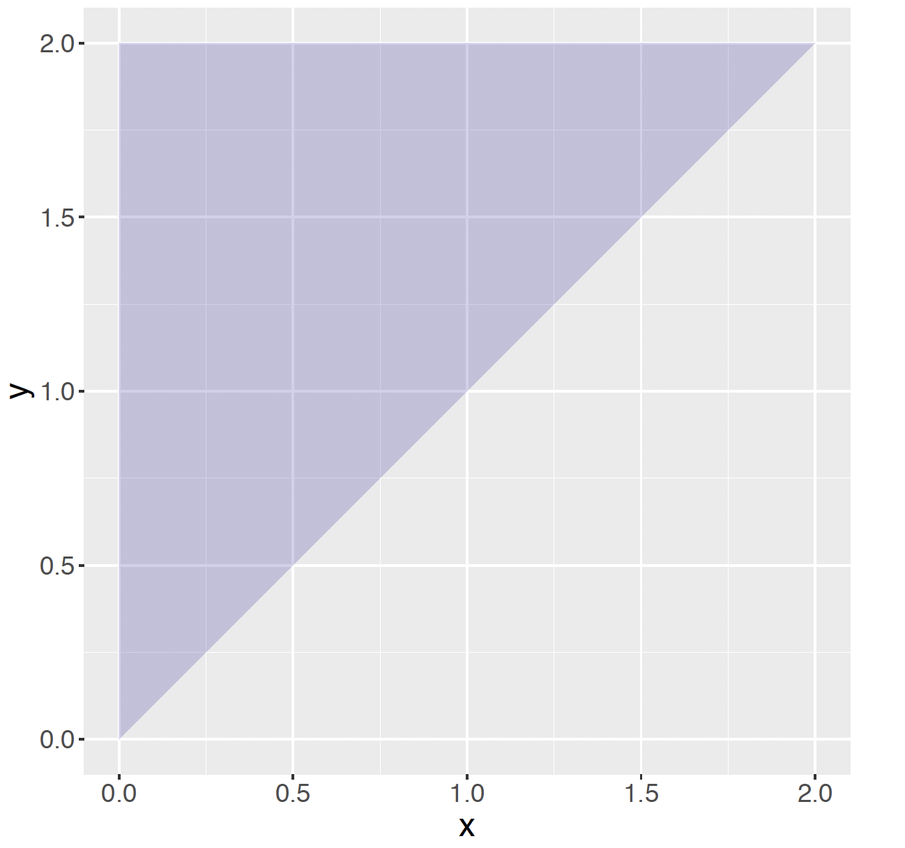
Figure 6.1: Region where the joint pdf \(f(x, y)\) is positive in the choose two points example.
This joint pdf is viewed as a plane of constant height over the set of points \((x, y)\) where \(0 < x < y <2\). This region of points in the plane is shown in Figure 6.1.
In the one variable situation in Chapter 5, a function \(f\) is a legitimate density function or pdf if it is nonnegative over the real line and the total area under the curve is equal t to one. Similarly for two variables, any function \(f(x, y)\) is considered a pdf if it satisfies two properties:
- Density is nonnegative over the whole plane: \[\begin{equation} f(x, y) \ge 0, \, \, {\rm for} \, {\rm all} \, \, x, y. \tag{6.5} \end{equation}\]
- The total volume under the density is equal to one: \[\begin{equation} \int \int f(x, y) dx dy = 1. \tag{6.6} \end{equation}\]
One can check that the pdf in our example is indeed a legitimate pdf. It is pretty obvious that the density that was defined is nonnegative, but it is less clear that the integral of the density is equal to one. Since the density is a plane of constant height, one computes this double integral geometrically. Using the familiar ``one half base times height" argument, the area of the triangle in the plane is \((1/2) (2) (2) = 2\) and since the pdf has constant height of \(1/2\), the volume under the surface is equal to \(2 (1/2) =1\).
Probabilities about \(X\) and \(Y\) are found by finding volumes under the pdf surface. For example, suppose one wants to find the probability that the sum of locations \(X + Y > 3\), that is \(P(X + Y > 3)\). The region in the \((x, y)\) plane of interest is first identified, and then one finds the volume under the joint pdf over this region.
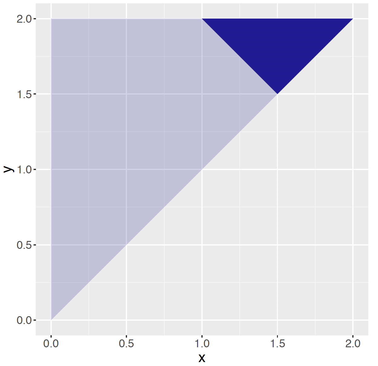
Figure 6.2: Shaded region where x + y > 3 in the choose two points example.
In Figure 6.2, the region where \(x + y > 3\) has been shaded. The probability \(P(X + Y > 3)\) is the volume under the pdf over this region. Applying a geometric argument, one notes that the area of the shaded region is \(1/4\), and so the probability of interest is \((1/4)(1/2) = 1/8\). One also finds this probability by integrating the joint pdf over the region as follows: \[\begin{align*} P(X + Y < 3) & = \int_{1.5}^2 \int^y_{3-y} f(x, y) dx dy \\ & = \int_{1.5}^2 \int^y_{3-y} \frac{1}{2} dx dy \\ & = \int_{1.5}^2 \frac{2 y - 3}{2}dy \\ & = \frac{y^2 - 3 y}{ 2} \Big|_{1.5}^2 \\ & = \frac{1}{8}. \end{align*}\]
Marginal probability density functions
Given a joint pdf \(f(x, y)\) that describes probabilities of two continuous variables \(X\) and \(Y\), one summarizes probabilities about each variable individually by the computation of marginal pdfs. The marginal pdf of \(X\), \(f_X(x)\), is obtained by integrating out \(y\) from the joint pdf. \[\begin{equation} f_X(x) = \int f(x, y) dy. \tag{6.7} \end{equation}\] In a similar fashion, one defines the marginal pdf of \(Y\) by integrating out \(x\) from the joint pdf. \[\begin{equation} f_Y(x) = \int f(x, y) dx. \tag{6.8} \end{equation}\]
Let’s illustrate the computation of marginal pdfs for our example. One has to be careful about the limits of the integration due to the dependence between \(x\) and \(y\) in the support of the joint density. Looking back at Figure 6.1, one sees that if the value of \(x\) is fixed, then the limits for \(y\) go from \(x\) to 2. So the marginal density of \(X\) is given by \[\begin{align*} f_X(x) & = \int f(x, y) dy \\ & = \int_x^2 \frac{1}{2} dy \\ & = \frac{2 - x}{2}, \, \, 0 < x < 2. \end{align*}\] By a similar calculation, one can verify that the marginal density of \(Y\) is equal to \[ f_Y(y) = \frac{y}{2}, \, \, 0 < y < 2. \]
Conditional probability density functions
Once a joint pdf \(f(x, y)\) has been defined, one can also define conditional pdfs. In our example, suppose one is told that the first random location is equal to \(X = 1.5\). What has one learned about the value of the second random variable \(Y\)?
To answer this question, one defines the notion of a conditional pdf. The conditional pdf of the random variable \(Y\) given the value \(X = x\) is defined as the quotient \[\begin{equation} f_{Y \mid X}(y \mid X = x) = \frac{f(x, y)}{f_X(x)}, \, \, {\rm if} \, \, f_X(x) > 0. \tag{6.9} \end{equation}\] In our example one is given that \(X = 1.5\). Looking at Figure 6.1, one sees that when \(X = 1.5\), the only possible values of \(Y\) are between 1.5 and 2. By substituting the values of \(f(x, y)\) and \(f_X(x)\), one obtains \[\begin{align*} f_{Y \mid X}(y \mid X = 1.5) & = \frac{f(1.5, y)}{f_X(1.5)} \\ & = \frac{1/2}{(2 - 1.5) / 2} \\ & = 2, \, \, 1.5 < y < 2. \\ \end{align*}\] In other words, the conditional density for \(Y\) when \(X = 1.5\) is uniform from 1.5 to 2.
A conditional pdf is a legitimate density function, so the integral of the pdf over all values \(y\) is equal to one. We use this density to compute conditional probabilities. For example, if \(X\) = 1.5, what is the probability that \(Y\) is greater than 1.7? This probability is the conditional probability \(P(Y > 1.7 \mid X = 1.5)\) that is equal to an integral over the conditional density \(f_{Y \mid X}(y \mid 1.5)\): \[\begin{align*} P(Y > 1.7 \mid X = 1.5) & = \int_{1.7}^2 f_{Y \mid X}(y \mid 1.5) dy \\ & = \int_{1.7}^2 2 dy \\ & = 0.6. \\ \end{align*}\]
Turn the random variables around
Above, we looked at the pdf of \(Y\) conditional on a value of \(X\). One can also consider a pdf of \(X\) conditional on a value of \(Y\). Returning to our example, suppose that one learns that \(Y\), the larger random variable on the interval is equal to 0.8. In this case, what would one expect for the random variable \(X\)?
This question is answered in two steps – one first finds the conditional pdf of \(X\) conditional on \(Y = 0.8\). Then once this conditional pdf is found, one finds the mean of this distribution.
The conditional pdf of \(X\) given the value \(Y = y\) is defined as the quotient \[\begin{equation} f_{X \mid Y}(x \mid Y = y) = \frac{f(x, y)}{f_Y(y)}, \, \, {\rm if} \, \, f_Y(y) > 0. \tag{6.10} \end{equation}\] Looking back at Figure 6.1, one sees that if \(Y = 0.8\), the possible values of \(X\) are from 0 to 0.8. Over these values the conditional pdf of \(X\) is given by \[\begin{align*} f_{X \mid Y}(x \mid 0.8) & = \frac{f(x, 0.8)}{f_Y(0.8)} \\ & = \frac{1/2}{0.8 / 2} \\ & = 1.25, \, \, 0 < x < 0.8. \\ \end{align*}\] So if one knows that \(Y = 0.8\), then the conditional pdf for \(X\) is Uniform on (0, 0.8).
To find the ``expected" value of \(X\) knowing that \(Y = 0.8\), one finds the mean of this distribution. \[\begin{align*} E(X \mid Y = 0.8) & = \int_0^{0.8} x f_{X \mid Y}(x \mid 0.8) dx \\ & = \int_0^{0.8} x \,1.25 \, dx \\ \\ & = (0.8)^2 / 2 \times 1.25 = 0.4. \\ \end{align*}\]
6.5 Independence and Measuring Association
As a second example, suppose one has two random variables (\(X, Y\)) that have the joint density \[ f(x, y) = \begin{cases} x + y, \, \, 0 < x < 1, 0 < y < 1;\\ 0, \, \,{\rm elsewhere}. \end{cases} \] This density is positive over the unit square, but the value of the density increases in \(X\) (for fixed \(y\)) and also in \(Y\) (for fixed \(x\)). Figure 6.3 displays a graph of this joint pdf – the density is a section of a plane that reaches its maximum value at the point (1, 1).
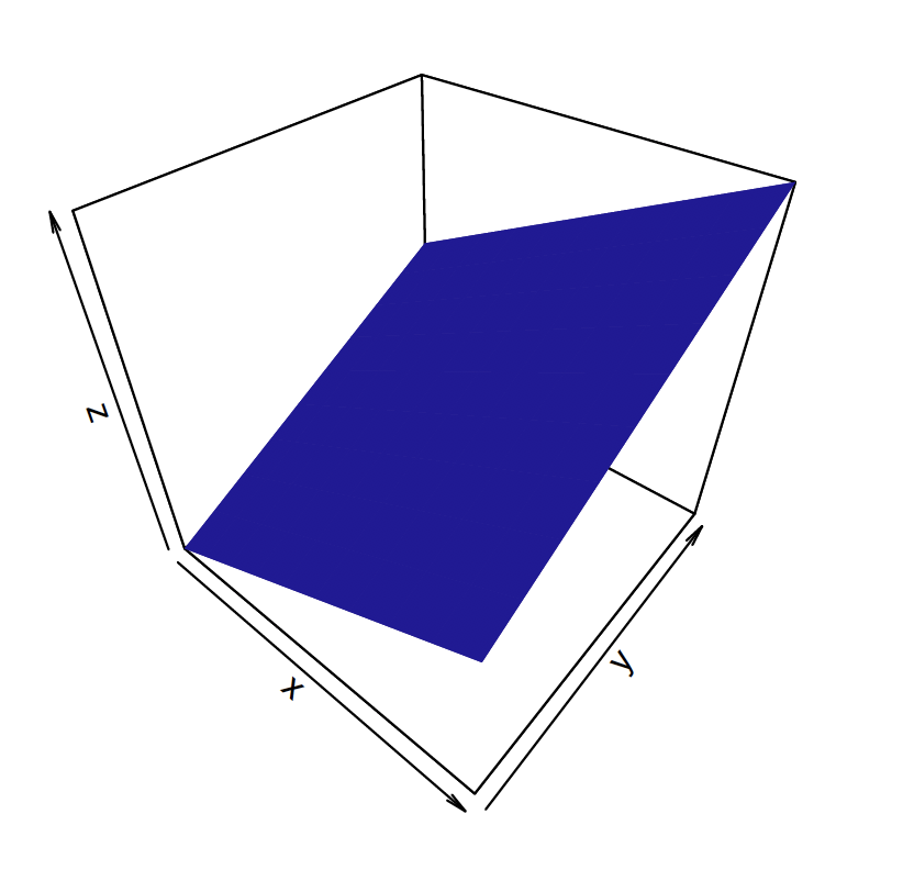
Figure 6.3: Three dimensional display of the pdf of f(x; y) = x + y defined over the unit square.
From this density, one computes the marginal pdfs of \(X\) and \(Y\). For example, the marginal density of \(X\) is given by \[\begin{align*} f_X(x) & = \int_0^1 x + y dy \\ & = x + \frac{1}{2}, \, \, \, 0 < x < 1. \\ \\ \end{align*}\] Similarly, one can show that the marginal density of \(Y\) is given by \(f_Y(y) = y + \frac{1}{2}\) for \(0 < y < 1\).
Independence
Two random variables \(X\) and \(Y\) are said to be independent if the joint pdf factors into a product of their marginal densities, that is \[\begin{equation} f(x, y) = f_X(x) f_Y(y). \tag{6.11} \end{equation}\] for all values of \(X\) and \(Y\). Are \(X\) and \(Y\) independent in our example? Since we have computed the marginal densities, we look at the product \[ f_X(x) f_Y(y) = (x + \frac{1}{2}) (y + \frac{1}{2}) \] which is clearly not equal to the joint pdf \(f(x, y) = x + y\) for values of \(x\) and \(y\) in the unit square. So \(X\) and \(Y\) are not independent in this example.
Measuring association by covariance
In the situation like this one where two random variables are not independent, it is desirable to measure the association pattern. A standard measure of association is the covariance defined as the expectation \[\begin{align} Cov(X, Y) & = E\left((X - \mu_X) (Y - \mu_Y)\right) \nonumber \\ & =\int \int (x - \mu_X)(y - \mu_Y) f(x, y) dx dy. \tag{6.12} \end{align}\] For computational purposes, one writes the covariance as \[\begin{align} Cov(X, Y) & = E(X Y) - \mu_X \mu_Y \nonumber \\ & = \int \int (x y) f(x, y) dx dy - \mu_X \mu_Y. \tag{6.13} \end{align}\]
For our example, one computes the expectation \(E(XY)\) from the joint density: \[\begin{align*} E(XY) & = \int_0^1 \int_0^1 (xy) (x + y) dx dy \\ & = \int \frac{y}{3} + \frac{y^2}{2} dy \\ & = \frac{1}{3}. \end{align*}\] One can compute that the means of \(X\) and \(Y\) are given by \(\mu_X = 7/12\) and \(\mu_Y = 7/12\), respectively. So then the covariance of \(X\) and \(Y\) is given by \[\begin{align*} Cov(X, Y) & = E(X Y) - \mu_X \mu_Y \\ & =\frac{1}{3} - \left(\frac{7}{12}\right) \left(\frac{7}{12}\right) \\ & = -\frac{1}{144}. \end{align*}\]
It can be difficult to interpret a covariance value since it depends on the scale of the support of the \(X\) and \(Y\) variables. One standardizes this measure of association by dividing by the standard deviations of \(X\) and \(Y\) resulting in the correlation measure \(\rho\): \[\begin{equation} \rho = \frac{Cov(X, Y)}{\sigma_X \sigma_Y}. \tag{6.14} \end{equation}\] In a separate calculation one can find the variances of \(X\) and \(Y\) to be \(\sigma_X^2 = 11/144\) and \(\sigma_Y^2 = 11/144\). Then the correlation is given by \[\begin{align*} \rho & = \frac{-1 / 144}{\sqrt{11/144}\sqrt{11/144}} \\ & = -\frac{1}{11}. \end{align*}\] It can be shown that the value of the correlation \(\rho\) falls in the interval \((-1, 1)\) where a value of \(\rho = -1\) or \(\rho = 1\) indicates that \(Y\) is a linear function of \(X\) with probability 1. Here the correlation value is a small negative value indicates weak negative association between \(X\) and \(Y\).
6.6 Flipping a Random Coin: The Beta-Binomial Distribution
Suppose one has a box of coins where the coin probabilities vary. If one selects a coin from the box, \(p\), the probability the coin lands heads follows the distribution \[ g(p) = \frac{1}{B(6, 6)} p^5 (1 - p)^5, \, \, 0 < p < 1, \] where \(B(6,6)\) is the Beta function, which will be more thoroughly discussed in Chapter 7. This density is plotted in Figure 6.4. A couple of things to notice about this density. First, the density has a significant height over much of the plausible values of the probability – this reflects the idea that one are really unsure about the chance of observing a heads when flipped. Second, the density is symmetric about \(p = 0.5\), which means that the coin is equally likely to be biased towards heads or biased towards tails.
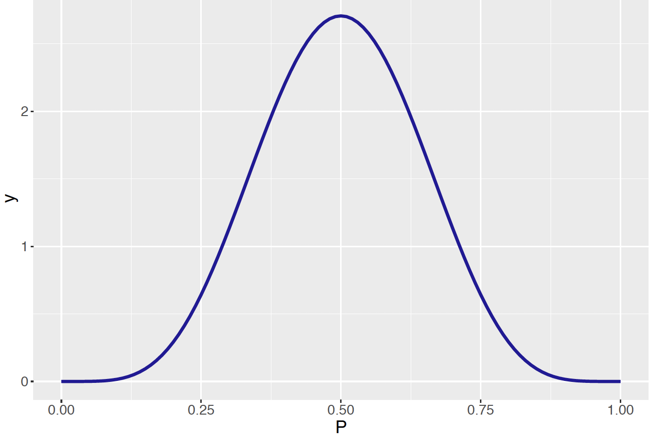
Figure 6.4: Beta(6, 6) density representing the distribution of probabilities of heads for a large collection of random coins.
One next flips this ``random" coin 20 times.
Denote the outcome of this experiment by the random variable \(Y\) which is equal to the count of heads. If we are given a value of the probability \(p\), then \(Y\) has a Binomial distribution with \(n = 20\) trials and success probability \(p\). This probability function is actually the conditional probability of observing \(y\) heads given a value of the probability \(p\):
\[
f(y \mid p) = {20 \choose y} p ^ y (1 - p) ^ {20 - y}, \, \, y = 0, 1, ..., 20.
\]
Given the density of \(p\) and the conditional density of \(Y\) conditional on \(p\), one computes the joint density by the product \[\begin{align*} f(y, p) = & \, g(p) f(y \mid p) = \left[ \frac{1}{B(6, 6)} p^5 (1 - p)^5\right] \left[{20 \choose y} p ^ y (1 - p) ^ {20 - y}\right] \\ = & \frac{1}{B(6, 6)} {20 \choose y} p^{y + 5} (1 - p)^{25 - y}, \, \, 0 < p < 1, y = 0, 1, ..., 20. \\ \end{align*}\] This is a mixed density in the sense that one variable (\(p\)) is continuous and one (\(Y\)) is discrete. This will not create any problems in the computation of marginal or conditional distributions, but one should be careful to understand the support of each random variable.
Simulating from the Beta-Binomial Distribution
Using R it is straightforward to simulate a sample of \((p, y)\) values from the Beta-Binomial distribution. Using the rbeta() function, one takes a random sample of 500 draws from the Beta(6, 6) distribution. Then for each probability value \(p\), one uses the rbinom() function to simulate the number of heads in 20 flips of this ``\(p\) coin."
library(ggplot2)
data.frame(p = rbeta(500, 6, 6)) %>%
  mutate(Y = rbinom(500, size = 20, prob = p)) -> df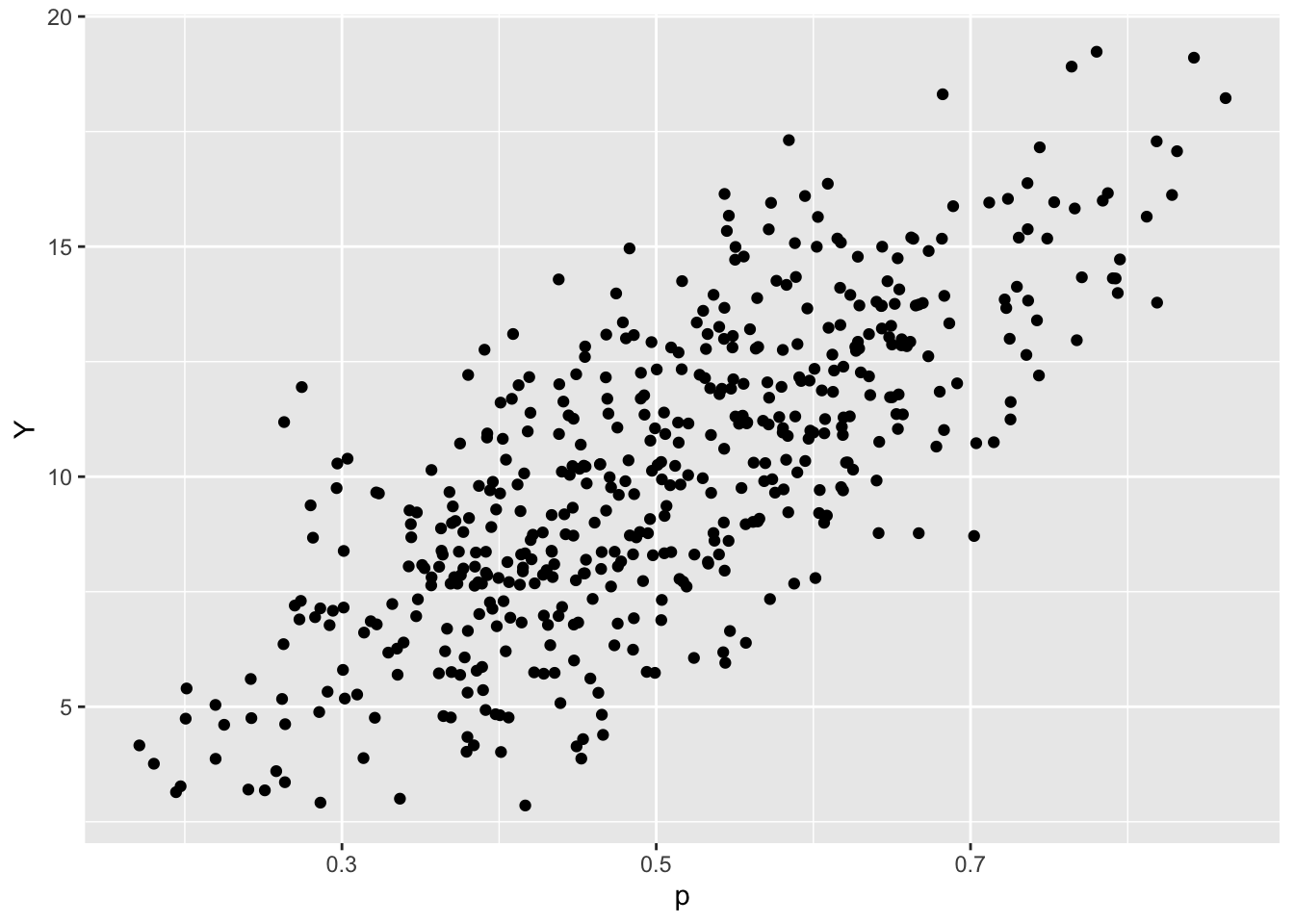
Figure 6.5: Scatterplot of 500 simulated draws from the joint density of the probability of heads \(p\) and the number of heads \(Y\) in 20 flips.
A scatterplot of the simulated values of \(p\) and \(Y\) is displayed in Figure 6.5. Note that the variables are positively correlated, which indicates that one tends to observe a large number of heads with coins with a large probability of heads.
What is the probability that one observes exactly 10 heads in the 20 flips, that is \(P(Y = 10)\)? One performs this calculation by computing the marginal probability function for \(Y\). This is obtained by integrating out the probability \(p\) from the joint density. This density is a special case of the Beta-Binomial distribution. \[\begin{align*} f(y) = & \, \int_0^1 g(p) f(y \mid p) dp \\ = & \int_0^1 \frac{1}{B(6, 6)} {20 \choose y} p^{y + 5} (1 - p)^{25 - y} dp\\ = & {20 \choose y} \frac{B(y + 6, 26 - y)}{B(6, 6)}, \, \, y = 0, 1, 2, ..., 20. \end{align*}\]
Using this formula with the substitution \(y = 10\), we use R to find the probability \(P(Y = 10)\).
## [1] 0.10650486.7 Bivariate Normal Distribution
Suppose one collects multiple body measurements from a group of 30 students. For example, for each of 30 students, one might collect the diameter of the wrist and the diameter of the ankle. If \(X\) and \(Y\) denote the two body measurements (measured in cm) for a student, then one might think that the density of \(X\) and the density of \(Y\) is each Normally distributed. Moreover, the two random variables would be positively correlated – if a student has a large wrist diameter, one would predict her to also have a large forearm length.
A convenient joint density function for two continuous measurements \(X\) and \(Y\), each variable measured on the whole real line, is the Bivariate Normal density with density given by \[\begin{equation} f(x, y) = \frac{1}{2 \pi \sigma_X \sigma_Y \sqrt{1 - \rho}} \exp\left[-\frac{1}{2 (1 - \rho^2)}(z_X^2 - 2 \rho z_X z_Y + z_Y^2)\right], \tag{6.15} \end{equation}\] where \(z_X\) and \(z_Y\) are the standardized scores \[\begin{equation} z_X = \frac{x - \mu_X}{\sigma_X}, \, \, \, z_Y = \frac{y - \mu_Y}{\sigma_Y}, \tag{6.16} \end{equation}\] and \(\mu_X, \mu_Y\) and \(\sigma_X, \sigma_Y\) are respectively the means and standard deviations of \(X\) and \(Y\). The parameter \(\rho\) is the correlation of \(X\) and \(Y\) and measures the association between the two variables.
Figure 6.6 shows contour plots of four Bivariate Normal distributions. The bottom right graph corresponds to the values \(\mu_X = 17, \mu_Y = 23, \sigma_X = 2, \sigma_Y = 3\) and \(\rho = 0.4\) where \(X\) and \(Y\) represent the wrist diameter and ankle diameter measurements of the student. The correlation value of \(\rho = 0.4\) reflects the moderate positive correlation of the two body measurements. The other three graphs use the same means and standard deviations but different values of the \(\rho\) parameter. This figure shows that the Bivariate Normal distribution is able to model a variety of association structures between two continuous measurements.
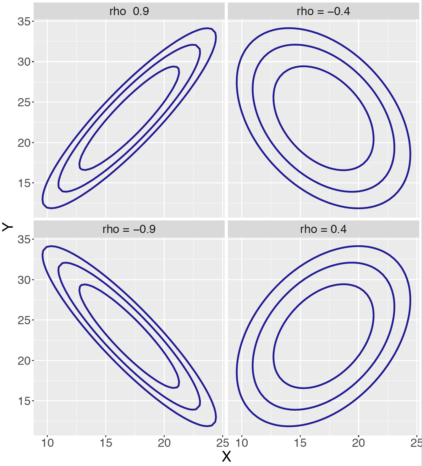
Figure 6.6: Contour graphs of four Bivariate Normal distributions with different correlations.
There are a number of attractive properties of the Bivariate Normal distribution.
The marginal densities of \(X\) and \(Y\) are Normal. So \(X\) has a Normal density with parameters \(\mu_X\) and \(\sigma_X\) and likewise \(Y\) is \(\textrm{Norma}(\mu_Y, \sigma_Y)\).
The conditional densities will also be Normal. For example, if one is given that \(Y = y\), then the conditional density of \(X\) given \(Y = y\) is Normal where
\[\begin{equation} E(X \mid Y = y) = \mu_X + \rho \frac{\sigma_X}{\sigma_Y}(y - \mu_Y), \, \, Var(X \mid Y = y) = \sigma_X^2(1 - \rho^2). \end{equation}\] Similarly, if one knows that \(X = x\), then the conditional density of \(Y\) given \(X = x\) is Normal with mean \(\mu_Y + \rho \frac{\sigma_Y}{\sigma_X}(x - \mu_X)\) and variance \(\sigma_Y^2(1 - \rho^2)\).
- For a Bivariate Normal distribution, \(X\) and \(Y\) are independent if and only if the correlation \(\rho = 0\). In contrast, as the correlation parameter \(\rho\) approaches \(+1\) and \(-1\), then all of the probability mass will be concentrated on a line where \(Y = a X + b\).
Bivariate Normal calculations
Returning to the body measurements application, different uses of the Bivariate Normal model can be illustrated. Recall that \(X\) denotes the wrist diameter, \(Y\) represents the ankle diameter and we are assuming \((X, Y)\) has a Bivariate Normal distribution with parameters \(\mu_X = 17, \mu_Y = 23, \sigma_X = 2, \sigma_Y = 3\) and \(\rho = 0.4\)
- Find the probability a student’s wrist diameter exceeds 20 cm.
Here one is interested in the probability \(P(X > 20)\). From the facts above, the marginal density for \(X\) will be Normal with mean \(\mu_X = 17\) and standard deviation \(\sigma_X = 2\). So this probability is computed using the function pnorm():
## [1] 0.0668072- Suppose one is told that the student’s ankle diameter is 20 cm – find the conditional probability \(P(X > 20 \mid Y = 20)\).
By above the distribution of \(X\) conditional on the value \(Y = y\) is Normal with mean \(\mu_X + \rho \frac{\sigma_X}{\sigma_Y}(y - \mu_Y)\) and variance \(\sigma_X^2(1 - \rho^2)\). Here one is conditioning on the value \(Y = 20\) and one computes the mean and standard deviation and apply the pnorm() function:
\[\begin{align*}
E(X \mid Y = 20) & = \mu_X + \rho \frac{\sigma_X}{\sigma_Y}(y - \mu_Y) \\
& = 17 + 0.4 \left(\frac{2}{3}\right)(20 - 23) \\
& = 16.2.
\end{align*}\]
\[\begin{align*}
SD(X \mid Y = 20) & = \sqrt{\sigma_X^2(1 - \rho^2)} \\
& = \sqrt{2^2 (1 - 0.4^2)} \\
& = 1.83.
\end{align*}\]
## [1] 0.01892374- Are \(X\) and \(Y\) independent variables?
By the properties above, for a Bivariate Normal distribution, a necessary and sufficient condition for independence is that the correlation \(\rho = 0\). Since the correlation between the two variables is not zero, the random variables \(X\) and \(Y\) can not be independent.
- Find the probability a student’s ankle diameter measurement is at 50 percent greater than her wrist diameter measurement, that is \(P(Y > 1.5 X)\).
Simulating Bivariate Normal measurements
The computation of the probability \(P(Y > 1.5 X)\) is not obvious from the information provided. But simulation provides an attractive method of computing this probability. One simulates a large number, say 1000, draws from the Bivariate Normal distribution and then finds the fraction of simulated \((x, y)\) pairs where \(y > 1.5 x\). Figure 6.7 displays a scatterplot of these simulated draws and the line \(y = 1.5 x\). The probability is estimated by the fraction of points that fall to the left of this line. In the R script below we use a function sim_binorm() to simulate 1000 draws from a Bivariate Normal distribution with inputted parameters \(\mu_X, \mu_Y, \sigma_X, \sigma_Y, \phi\). The bivariate normal parameters are set to the values in this example and using the function sim_binorm() the probability of interest is approximated by 0.242.
sim_binorm <- function(mx, my, sx, sy, r){
  require(ProbBayes)
  v <- matrix(c(sx ^ 2, r * sx * sy,
                r * sx * sy, sy ^ 2),
                2, 2)
  as.data.frame(rmnorm(1000, mean = c(mx, my),
                       varcov = v))}
mx <- 17; my <- 23; sx <- 2; sy <- 3; r <- 0.4
sdata <- sim_binorm(mx, my, sx, sy, r)
names(sdata) <- c("X", "Y")
sdata %>% summarize(mean(Y > 1.5 * X))
## mean(Y > 1.5 * X)
## 1 0.218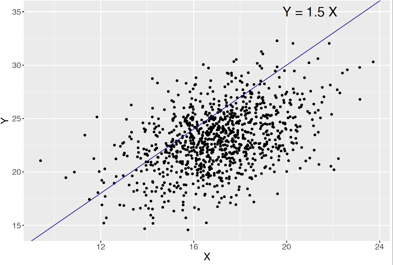
Figure 6.7: Scatterplot of simulated draws from the Bivariate Normal in body measurement example. The probability that \(Y > 1.5 X\) is approximated by the proportion of simulated points that fall to the left of the line \(y = 1.5 x\).
6.8 Exercises
- Coin Flips
Suppose you flip a coin three times with eight equally likely outcomes \(HHH, HHT, ..., TTT\). Let \(X\) denote the number of heads in the first two flips and \(Y\) the number of heads in the last two flips.
- Find the joint probability mass function (pmf) of \(X\) and \(Y\) and put your answers in the following table.
| y | |||
|---|---|---|---|
| \(x\) | 0 | 1 | 2 |
| 0 | |||
| 1 | |||
| 2 |
- Find \(P(X > Y)\).
- Find the marginal pmf’s of \(X\) and \(Y\).
- Find the conditional pmf of \(X\) given \(Y = 1\).
- Selecting Numbers
Suppose you select two numbers without replacement from the set {1, 2, 3, 4, 5}. Let \(X\) denote the smaller of the two numbers and \(Y\) denote the larger of the two numbers.
- Find the joint probability mass function of \(X\) and \(Y\).
- Find the marginal pmf’s of \(X\) and \(Y\).
- Are \(X\) and \(Y\) independent? If not, explain why.
- Find \(P(Y = 3 \mid X = 2)\).
- Die Rolls
You roll a die 4 times and record \(O\), the number of ones, and \(T\) the number of twos rolled.
- Construct the joint pmf of \(O\) and \(T\).
- Find the probability \(P(O = T)\).
- Find the conditional pmf of \(T\) given \(O = 1\).
- Compute \(P(T > 0 \mid O = 1)\).
- Choosing Balls
Suppose you have a box with 3 red and 2 black balls. You first roll a die – if the roll is 1, 2, you sample 3 balls without replacement from the box. If you roll is 3 or higher, you sample 2 balls without replacement from the box. Let \(X\) denote the number of balls you sample and \(Y\) the number of red balls selected.
- Find the joint pmf of \(X\) and \(Y\).
- Find the probability \(P(X = Y)\).
- Find the marginal pmf of \(Y\).
- Find the conditional pmf of \(X\) given \(Y = 2\).
- Baseball Hitting
Suppose a player is equally likely to have 4, 5, or 6 at-bats (opportunities) in a baseball game. If \(N\) is the number of opportunities, then assume that \(X\), the number of hits, is Binomial with probability \(p = 0.3\) and sample size \(N\).
- Find the joint pmf of \(N\) and \(X\).
- Find the marginal pmf of \(X\).
- Find the conditional pmf of \(N\) given \(X = 2\).
- If the player gets 3 hits, what is the probability he had exactly 5 at-bats?
- Multinomial Density
Suppose a box contains 4 red, 3 black, and 3 green balls. You sample eight balls with replacement from the box and let \(R\) denote the number of red and \(B\) the number of black balls selected.
- Explain why this is a Multinomial experiment and given values of the parameters of the Multinomial distribution for \((R, B)\).
- Compute \(P(R = 3, B = 2)\).
- Compute the probability that you sample more red balls than black balls.
- Find the marginal distribution of \(B\).
- If you are given that you sampled \(B = 4\) balls, find the probability that you sampled at most 2 red balls.
- Joint Density
Let \(X\) and \(Y\) have the joint density \[ f(x, y) = k y, \, \, 0 < x < 2, 0 < y < 2. \]
- Find the value of \(k\) so that \(f()\) is a pdf.
- Find the marginal density of \(X\).
- FInd \(P(Y > X)\).
- Find the conditional density of \(Y\) given \(X = x\) for any value \(0 < x < 2\).
- Joint Density
Let \(X\) and \(Y\) have the joint density \[ f(x, y) = x + y, \, \, 0 < x < 1, 0 < y < 1. \]
- Check that \(f\) is indeed a valid pdf. If it is not, correct the definition of \(f\) so it is valid.
- Find the probability \(P(X > 0.5, Y < 0.5)\).
- Find the marginal density of \(X\).
- Are \(X\) and \(Y\) independent? Answer by a suitable calculation.
- Random Division
Suppose one randomly chooses a values \(X\) on the interval (0, 2), and then random choosing a second point \(Y\) from 0 to \(X\).
- Find the joint density of \(X\) and \(Y\).
- Are \(X\) and \(Y\) independent? Explain.
- Find the probability \(P(Y > 0.5)\).
- Find the probability \(P(X + Y > 2)\).
- Choosing a Random Point in a Circle
Suppose (\(X, Y\)) denotes a random point selected over the unit circle. The joint pdf of (\(X, Y\)) is given by \[ f(x, y) = \begin{cases} C, \, \, x^2 + y^2 \le 1;\\ 0, \, \,{\rm elsewhere}. \end{cases} \]
- Find the value of the constant \(C\) so \(f()\) is indeed a joint pdf.
- Find the marginal pdf of \(Y\).
- Find the probability \(P(Y > 0.5)\)
- Find the conditional pdf of \(X\) conditional on \(Y = 0.5\).
- A Random Meeting
Suppose John and Jill independently arrive at an airport at a random between 3 and 4 pm one afternoon. Let \(X\) and \(Y\) denote respectively the number of minutes past 3 pm that John and Jill arrive.
- Find the joint pdf of \(X\) and \(Y\).
- Find the probability that John arrives later than Jill.
- Find the probability that John and Jill meet within 10 minutes of each other.
- Defects in Fabric
Suppose the number of defects per yard in a fabric \(X\) is assumed to have a Poisson distribution with mean \(\lambda\). That is, the conditional density of \(X\) given \(\lambda\) has the form \[ f(x \mid \lambda) = \frac{e^{-\lambda} \lambda^x}{x!}, x = 0, 1, 2, ... \] The parameter \(\lambda\) is assumed to be uniformly distributed over the values 0.5, 1, 1.5, and 2.
- Write down the joint pmf of \(X\) and \(\lambda\).
- Find the probability that the number of defects \(X\) is equal to 0.
- Find the conditional pmf of \(\lambda\) if you know that \(X = 0\).
- Defects in Fabric (continued)
Again we assume the number of defects per yard in a fabric \(X\) given \(\lambda\) has a Poisson distribution with mean \(\lambda\). But now we assume \(\lambda\) is continuous-valued with the exponential density \[ g(\lambda) = \exp(-\lambda), \, \, \lambda > 0. \]
Write down the joint density of \(X\) and \(\lambda\).
Find the marginal density of \(X\). [Hint: it may be helpful to use the integral identity \[ \int_0^\infty \exp(-a \lambda) \lambda^b d\lambda = \frac{b!}{a ^ {b + 1}}, \] where \(b\) is a nonnegative integer.]
Find the probability that the number of defects \(X\) is equal to 0.
Find the conditional density of \(\lambda\) if you know that \(X = 0\).
- Flipping a Random Coin
Suppose you plan flipping a coin twice where the probability \(p\) of heads has the density function \[ f(p) = 6 p (1 - p), \, \, 0 < p < 1. \] Let \(Y\) denote the number of heads of this “random” coin. \(Y\) given a value of \(p\) is Binomial with \(n = 2\) and probability of success \(p\).
- Write down the joint density of \(Y\) and \(p\).
- Find \(P(Y = 2)\).
- If \(Y = 2\), then find the probability that \(p\) is greater than 0.5.
- Passengers on An Airport Limousine
An airport limousine can accommodate up to four passengers on any one trip. The company will accept a maximum of six reservations for a trip, and a passenger must have a reservation. From previous records, \(30\%\) of all those making reservations do not appear for the trip. Answer the following questions, assuming independence whenever appropriate.
If six reservations are made, what is the probability that at least one individual with a reservation cannot be accommodated on the trip?
If six reservations are made, what is the expected number of available places when the limousine departs?
Suppose the probability distribution of the number of reservations made is given in the following table.
| Number of observations | 3 | 4 | 5 | 6 |
|---|---|---|---|---|
| Probability | 0.13 | 0.18 | 0.35 | 0.34 |
Let \(X\) denote the number of passengers on a randomly selected trip. Obtain the probability mass function of \(X\).
| \(x\) | 0 | 1 | 2 | 3 | 4 |
|---|---|---|---|---|---|
| \(p(x)\) |
- Heights of Fathers and Sons
It is well-know that heights of fathers and sons are positively association. In fact, if \(X\) represents the father’s height in inches and \(Y\) represents the son’s height, then the joint distribution of \((X, Y)\) can be approximated by a Bivariate Normal with means \(\mu_X = \mu_Y = 69\), \(\sigma_X = \sigma_Y = 3\) and correlation \(\rho = 0.4\).
- Are \(X\) and \(Y\) independent? Why or why not?
- Find the conditional density of the sons height if you know the father’s height is 70 inches.
- Using the result in part (b) to find \(P(Y > 72 \mid X = 70)\).
- By simulating from the Bivariate Normal distribution, approximate the probability that the son will be more than one inch taller than his father.
- Instruction and Students’ Scores
Twenty-two children are given a reading comprehension test before and after receiving a particular instruction method. Assume students’ pre-instructional and post-instructional scores follow a Bivariate Normal distribution with: \(\mu_{pre} = 47, \mu_{post} = 53, \sigma_{pre} = 13, \sigma_{post} = 15\) and \(\rho = 0.7\).
Find the probability that a student’s post-instructional score exceeds 60.
Suppose one student’s pre-instructional score is 45, find the probability that this student’s post-instructional score exceeds 70.
Find the probability that a student has increased the test score by at least 10 points. [Hint: Use R to simulate a large number of draws from the Bivariate Normal distribution. Refer to the example function in Section 6.7 for simulating Bivariate Normal draws.]
- Shooting Free Throws
Suppose a basketball player will take \(N\) free throw shots during a game where \(N\) has the following discrete distribution.
| \(N\) | 5 | 6 | 7 | 8 | 9 | 10 |
|---|---|---|---|---|---|---|
| Probability | 0.2 | 0.2 | 0.2 | 0.2 | 0.1 | 0.1 |
If the player takes \(N = n\) shots, then the number of makes \(Y\) is Binomial with sample size \(n\) and probability of success \(p = 0.7\).
Find the probability the player takes 6 shots and makes 4 of them.
From the joint distribution of \((N, Y)\), find the most likely \((n, y)\) pair.
Find the conditional distribution of the number of shots \(N\) if he makes 4 shots.
Find the expectation \(E(N \mid Y = 4)\).
- Flipping a Random Coin
Suppose one selects a probability \(p\) Uniformly from the interval (0, 1), and then flips a coin 10 times, where the probability of heads is the probability \(p\). Let \(X\) denote the observed number of heads.
Find the joint distribution of \(p\) and \(X\).
Use R to simulate a sample of size 1000 from the joint distribution of \((p, X)\).
From inspecting a histogram of the simulated values of \(X\), guess at the marginal distribution of \(X\).
R Exercises
- Simulating Multinomial Probabilities
Revisit Exercise 6.
Write an R function to simulate 10 balls drawn with replacement from the special weighted box (4 red, 3 black, and 3 green balls). [Hint: Section 6.3 introduces the function for the example of a special weighted die.]
Use the function to simulate the Multinomial experiment in Exercise 6 for 5000 iterations, and approximate \(P(R = 3, B = 2)\).
Use the 5000 simulated Multinomial experiments to approximate the probability that you sample more red balls than black balls, i.e. \(P(R > B)\).
Conditional on \(B = 4\), approximate the mean number of red balls will get sampled. Compare the approximated mean value to the exact mean. [Hint: Conditional on \(B = 4\), the distribution of \(R\) is a Binomial distribution.]
- Simulating from a Beta-Binomial Distribution
Consider a box of coins where the coin probabilities vary, and the probability of a selected coin lands heads, \(p\), follows a \(\textrm{Beta}(2, 8)\) distribution. Jason then continues to flip this ``random" coin 10 times, and is interested in the count of heads of the 10 flips, denoted by \(Y\).
Write an R function to simulate 5000 samples of \((p, y)\). [Hint: Use
rbeta()andrbinom()functions accordingly.]Approximate the probability that Jason observes 3 heads out of 10 flips, using the simulated 5000 samples. Compare the approximated probability to the exact probability. [Hint: Write out \(f(y)\) following the work in Section 6.6, and use R to calculate the exact probability.]
- Shooting Free Throws (continued)
Consider the free throws shooting in Exercise 18.
Write an R function to simulate 5000 samples of \((n, y)\).
From the 5000 samples, find the most likely \((n ,y)\) pair. Compare your result to Exercise 18 part (b).
Approximate the expectation \(E(N \mid Y = 4)\), and compare your result to Exercise 18 part (d).