Chapter 7 Hierarchical Modeling

7.1 Introduction to Hierarchical Modeling

library(LearnBayes)
library(lattice)

Fit logistic model for home run data for a particular player

logistic.fit <- function(player){
  d <- subset(sluggerdata, Player==player)
  x <- d$Age
  x2 <- d$Age^2
  response <- cbind(d$HR, d$AB - d$HR)
  list(Age=x,
       p=glm(response ~ x + x2,
             family=binomial)$fitted)
}

names <- unique(sluggerdata$Player)
newdata <- NULL
for (j in 1:9){
  fit <-logistic.fit(as.character(names[j]))
  newdata <- rbind(newdata,
            data.frame(as.character(names[j]),
                       fit$Age, fit$p))
}
names(newdata) <- c("Player", "Age", "Fitted")
xyplot(Fitted ~ Age | Player, 
       data=newdata, 
       type="l", lwd=3, col="black")

7.2 Individual or Combined Estimates

with(hearttransplants,
      plot(log(e), y / e, xlim=c(6, 9.7),
           xlab="log(e)", ylab="y/e"))
 with(hearttransplants,
      text(log(e), y / e,
           labels=as.character(y), pos=4))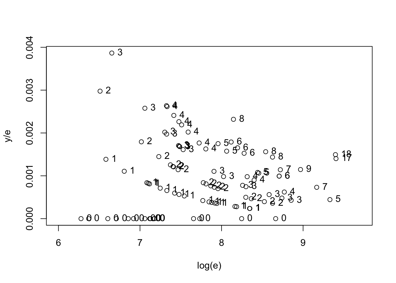

7.3 Equal Mortality Rates?

Using posterior predictive checks to see if equal mortality rate model is appropriate.

with(hearttransplants, sum(y))

## [1] 277

with(hearttransplants, sum(e))

## [1] 294681

lambda <- rgamma(1000, shape=277, rate=294681)
ys94 <- with(hearttransplants,
      rpois(1000, e[94] * lambda))

hist(ys94, breaks=seq(0.5, max(ys94) + 0.5))
with(hearttransplants,
      lines(c(y[94], y[94]), c(0, 120), lwd=3))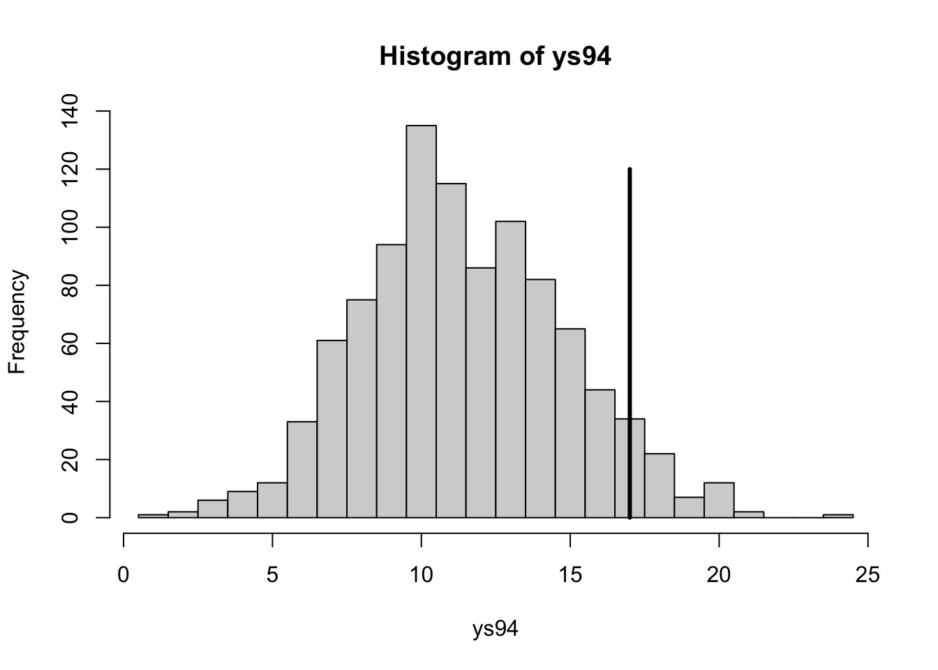

Find posterior predictive distribution of each observation with its posterior predictive distribution.

lambda <- rgamma(1000, shape=277, rate=294681)
prob.out <- function(i){
   ysi <- with(hearttransplants,
            rpois(1000, e[i] * lambda))
   pleft <- with(hearttransplants,
              sum(ysi <= y[i]) / 1000)
   pright <- with(hearttransplants,
               sum(ysi >= y[i]) / 1000)
   min(pleft, pright)
 }
pout <- sapply(1:94, prob.out)

with(hearttransplants,
     plot(log(e), pout, ylab="Prob(extreme)"))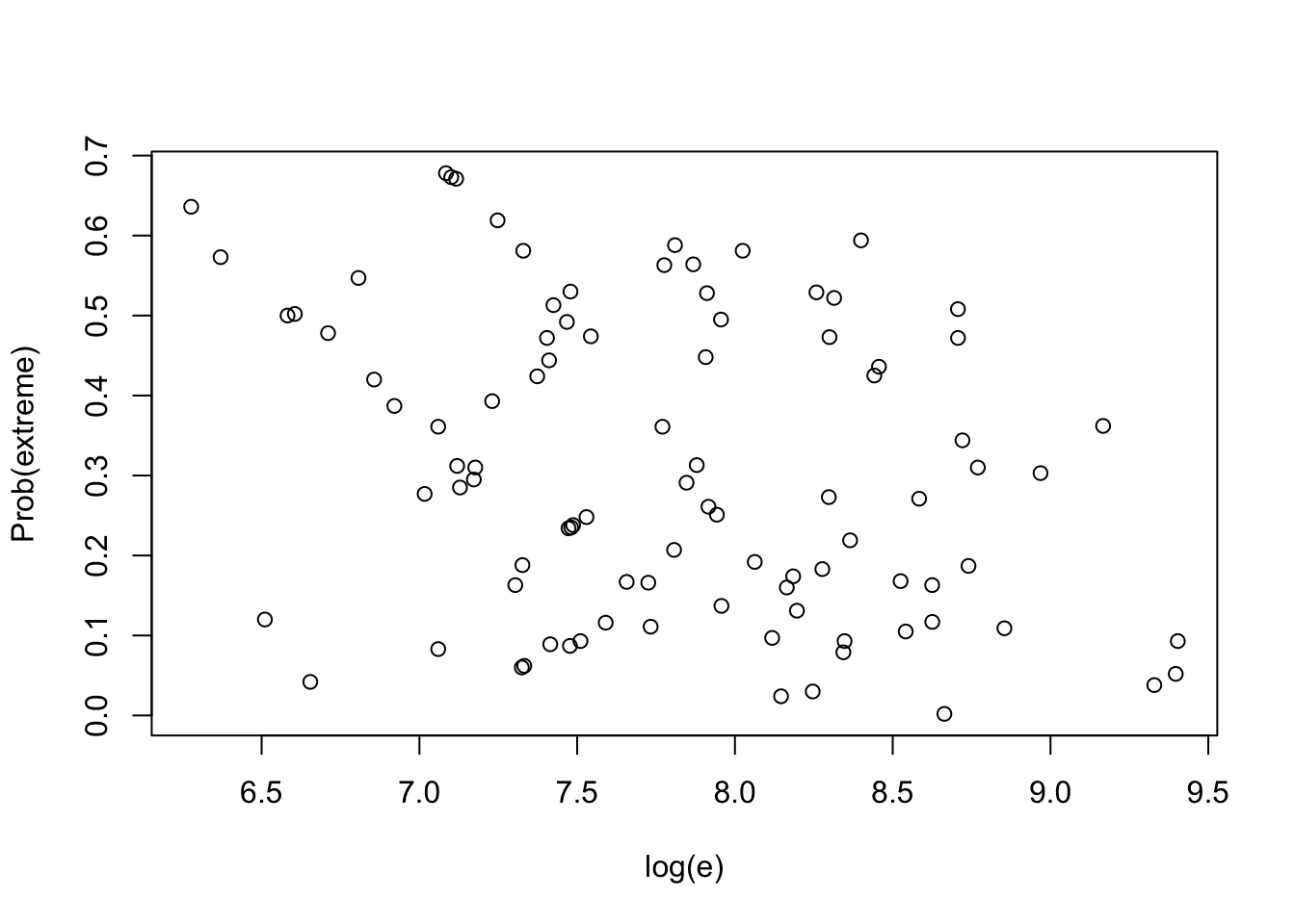

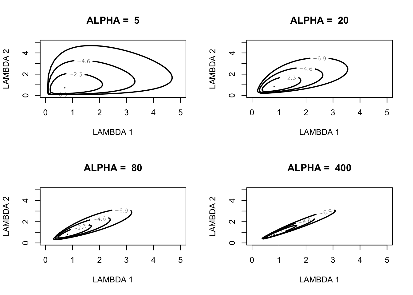
7.4 Modeling a Prior Belief of Exchangeability

Graph of two-stage prior to model a belief in exchangeability of the Poisson rates.

pgexchprior <- function(lambda, pars){
alpha <- pars[1]
a <- pars[2]
b <- pars[3]
(alpha - 1) * log(prod(lambda)) - 
  (2 * alpha + a) * log(alpha * sum(lambda) + b)
}

alpha <- c(5, 20, 80, 400)
par(mfrow=c(2, 2))
for (j in 1:4){
    mycontour(pgexchprior,
              c(.001, 5, .001, 5),
              c(alpha[j], 10, 10),
          main=paste("ALPHA = ",alpha[j]),
         xlab="LAMBDA 1", ylab="LAMBDA 2")
}

7.5 Simulating from the Posterior

Representing posterior as [\(\mu, \alpha\)] [\(\{\lambda_j\} | \mu, \alpha\)].

Focus on posterior of [\(\mu, \alpha\)]:

datapar <- list(data = hearttransplants, z0 = 0.53)
start <- c(2, -7)
fit <- laplace(poissgamexch, start, datapar)
 fit

## $mode
## [1]  1.883954 -6.955446
## 
## $var
##              [,1]         [,2]
## [1,]  0.233694921 -0.003086655
## [2,] -0.003086655  0.005866020
## 
## $int
## [1] -2208.503
## 
## $converge
## [1] TRUE

par(mfrow = c(1, 1))
mycontour(poissgamexch, c(0, 8, -7.3, -6.6),
          datapar,
          xlab="log alpha", ylab="log mu")

start <- c(4, -7)
fitgibbs <- gibbs(poissgamexch, 
                  start, 1000, 
                  c(1, .15), datapar)
fitgibbs$accept

##      [,1]  [,2]
## [1,] 0.52 0.483

mycontour(poissgamexch, 
         c(0, 8, -7.3, -6.6), 
         datapar,
         xlab="log alpha", ylab="log mu")
points(fitgibbs$par[, 1], fitgibbs$par[, 2])

plot(density(fitgibbs$par[, 1], bw = 0.2))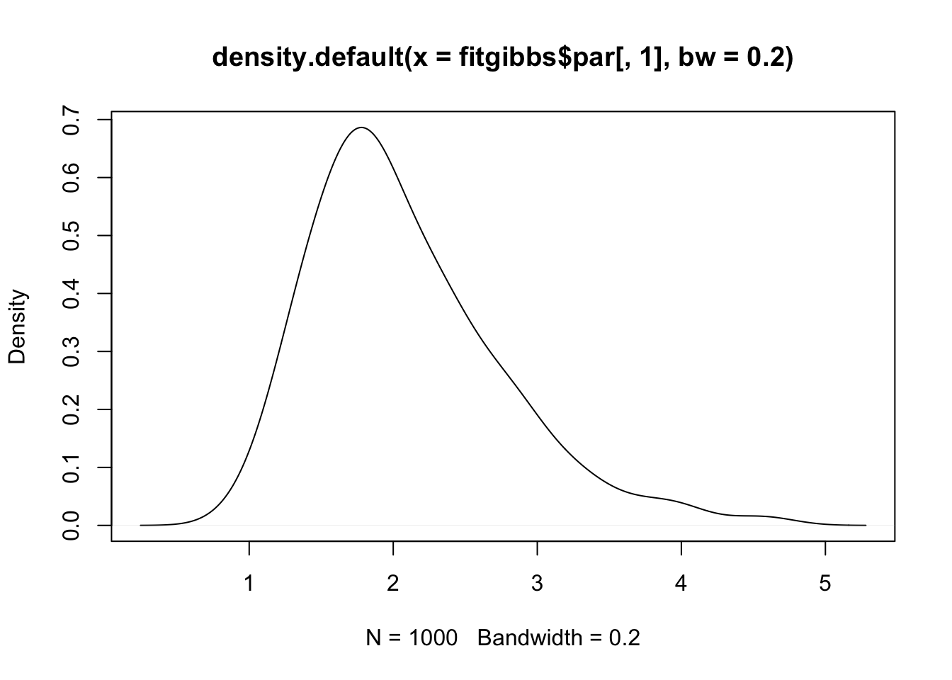

Posterior of rates:

alpha <- exp(fitgibbs$par[, 1])
mu <- exp(fitgibbs$par[, 2])
lam1 <- rgamma(1000, y[1] + alpha, 
               hearttransplants$e[1] + alpha / mu)
alpha <- exp(fitgibbs$par[, 1])
mu <- exp(fitgibbs$par[, 2])

with(hearttransplants,
     plot(log(e), y/e, pch = as.character(y)))
 for (i in 1:94) {
     lami <- with(hearttransplants,
           rgamma(1000, y[i] + alpha, 
               e[i] + alpha/mu))
     probint <- quantile(lami, c(0.05, 0.95))
     with(hearttransplants,
          lines(log(e[i]) * c(1, 1), probint))
 }

7.6 Posterior Inferences

datapar <- list(data = hearttransplants, z0 = 0.53)
start <- c(2, -7)
fit <- laplace(poissgamexch, start, datapar)
fit

## $mode
## [1]  1.883954 -6.955446
## 
## $var
##              [,1]         [,2]
## [1,]  0.233694921 -0.003086655
## [2,] -0.003086655  0.005866020
## 
## $int
## [1] -2208.503
## 
## $converge
## [1] TRUE

par(mfrow = c(1, 1))
mycontour(poissgamexch, 
          c(0, 8, -7.3, -6.6), datapar,
          xlab="log alpha",ylab="log mu")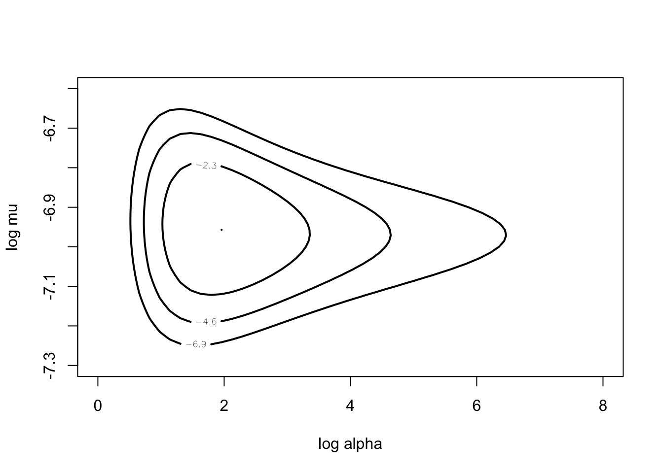

start <- c(4, -7)
fitgibbs <- gibbs(poissgamexch, 
                  start, 1000, 
                  c(1,.15), datapar)

alpha <- exp(fitgibbs$par[, 1])
mu <- exp(fitgibbs$par[, 2])

Look at posteriors of shrinkages.

shrink <-function(i)
with(hearttransplants,
       mean(alpha / (alpha + e[i] * mu)))
shrinkage=sapply(1:94, shrink)

with(hearttransplants,
     plot(log(e), shrinkage))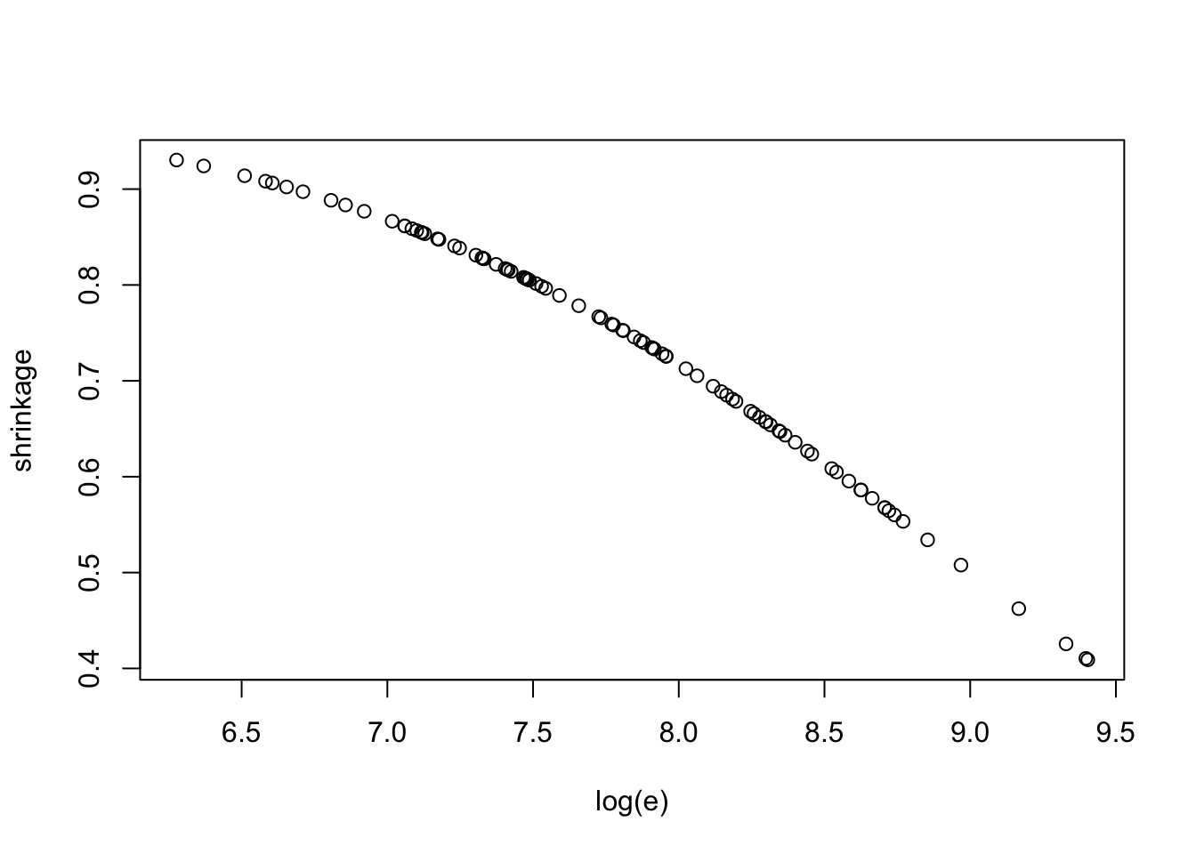

Comparing hospitals.

mrate <- function(i){
   with(hearttransplants,
       mean(rgamma(1000, y[i] + alpha, 
                  e[i] + alpha/mu)))
}
hospital <- 1:94
meanrate <- sapply(hospital,mrate)
hospital[meanrate == min(meanrate)]

## [1] 85

sim.lambda <- function(i) {
  with(hearttransplants,
       rgamma(1000, y[i] + alpha, 
              e[i] + alpha / mu))
}
LAM <- sapply(1:94, sim.lambda)

compare.rates <- function(x) {
  nc <- NCOL(x)
  ij <- as.matrix(expand.grid(1:nc, 1:nc))
  m <- as.matrix(x[,ij[,1]] > x[,ij[,2]])
  matrix(colMeans(m), nc, nc, byrow = TRUE)
}

better <- compare.rates(LAM)

better[1:24, 85]

##  [1] 0.174 0.190 0.086 0.144 0.124 0.227 0.203 0.166 0.067 0.255 0.196 0.176
## [13] 0.202 0.097 0.070 0.231 0.239 0.088 0.258 0.185 0.166 0.152 0.057 0.087

7.7 Bayesian Sensitivity Analysis

Explore sensitivity of inference with respect to the choice of \(z_0\) in prior.

datapar <- list(data = hearttransplants, 
                z0 = 0.53)

start <- c(4, -7)
fitgibbs <-gibbs(poissgamexch, 
                 start, 1000, 
                 c(1,.15), datapar)

sir.old.new <- function(theta, prior, prior.new){
  log.g <- log(prior(theta))
  log.g.new <- log(prior.new(theta))
  wt <- exp(log.g.new - log.g -
              max(log.g.new - log.g))
  probs <- wt / sum(wt)
  n <- length(probs)
  indices <- sample(1:n, size=n, 
                    prob=probs, replace=TRUE)
  theta[indices]
}

prior <- function(theta){
  0.53 * exp(theta) / (exp(theta) + 0.53) ^ 2
}
prior.new <- function(theta){
  5 * exp(theta) / (exp(theta) + 5) ^ 2
}

log.alpha <- fitgibbs$par[, 1]
log.alpha.new <- sir.old.new(log.alpha, 
                             prior, prior.new)

library(lattice)

draw.graph <- function(){
  LOG.ALPHA <- data.frame("prior", log.alpha)
  names(LOG.ALPHA) <- c("Prior", "log.alpha")
  LOG.ALPHA.NEW <- data.frame("new.prior",
                              log.alpha.new)
  names(LOG.ALPHA.NEW) <- c("Prior","log.alpha")
  D <- densityplot(~ log.alpha,
            group=Prior,
            data = rbind(LOG.ALPHA, LOG.ALPHA.NEW),
            plot.points=FALSE,
        main="Original Prior and Posterior (solid), \nNew Prior and Posterior (dashed)",
        lwd=4, adjust=2, lty=c(1,2),
        xlab="log alpha",xlim=c(-3,5),col="black")
    update(D, panel=function(...){
      panel.curve(prior(x), lty=1, lwd=2,
                  col="black")
      panel.curve(prior.new(x), lty=2, lwd=2,
                  col="black")
    panel.densityplot(...)
})}

draw.graph()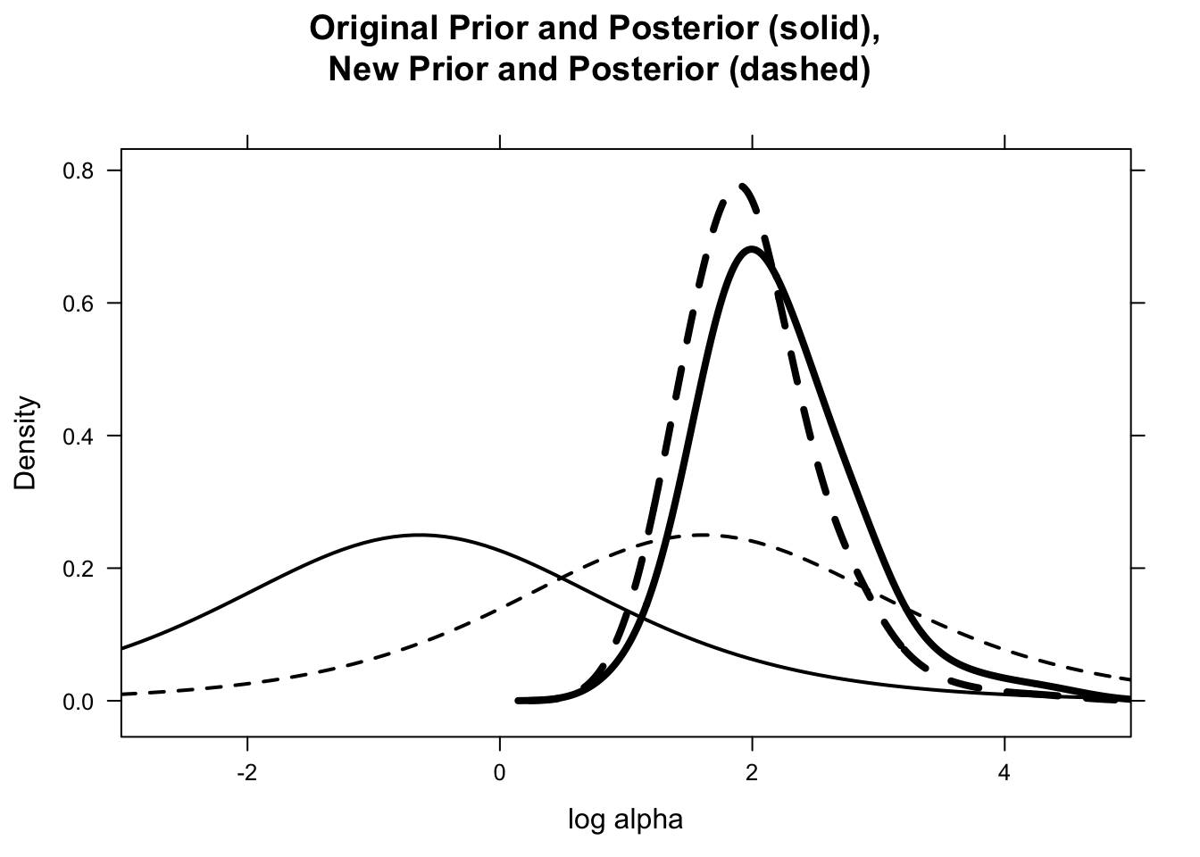

7.8 Posterior Predictive Model Checking

Study predictive distributions of observations.

datapar <- list(data = hearttransplants, z0 = 0.53)

start <- c(4, -7)
fitgibbs <- gibbs(poissgamexch, 
                  start, 1000, c(1,.15), 
                  datapar)

lam94 <- with(hearttransplants,
      rgamma(1000, y[94] + alpha, 
             e[94] + alpha / mu))

ys94 <- with(hearttransplants,
           rpois(1000, e[94] * lam94))

hist(ys94, breaks=seq(-0.5, max(ys94) + 0.5))
lines(y[94] * c(1, 1), c(0, 100), lwd=3)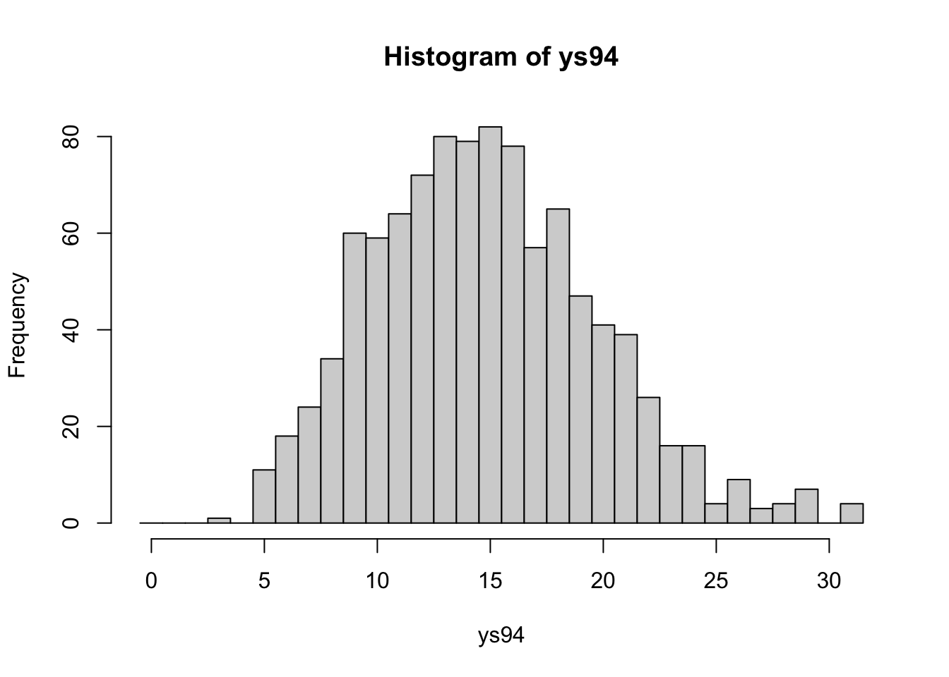

Explore the probabilities that the predictive distribution of each observation is at least as large as observed \(y_i\).

prob.out <- function(i){
   lami <- with(hearttransplants,
      rgamma(1000, y[i] + alpha, 
             e[i] + alpha / mu))
   ysi <- with(hearttransplants,
      rpois(1000, e[i] * lami))
   pleft <- with(hearttransplants,
      sum(ysi <= y[i]) / 1000)
   pright <- with(hearttransplants,
      sum(ysi >= y[i]) / 1000)
   min(pleft, pright)
 }
pout.exchange <- sapply(1:94, prob.out)

plot(pout, pout.exchange,
     xlab="P(extreme), equal means",
     ylab="P(extreme), exchangeable")
abline(0,1)