Chapter 4 Multiparameter Models

4.1 Normal Data with Both Parameters Unknown

Illustrates exact posterior sampling of (\(\mu, \sigma^2\)) for normal sampling with a noninformative prior.

library(LearnBayes)

mycontour(normchi2post, 
               c(220, 330, 500, 9000), 
               marathontimes$time,
               xlab="mean", ylab="variance")

S <- with(marathontimes, 
          sum((time - mean(time))^2))
n <- length(marathontimes$time)
sigma2 <- S / rchisq(1000, n - 1)
mu <- rnorm(1000, mean = mean(marathontimes$time),
            sd = sqrt(sigma2) / sqrt(n))
mycontour(normchi2post, 
               c(220, 330, 500, 9000), 
               marathontimes$time,
               xlab="mean", ylab="variance")
points(mu, sigma2)

quantile(mu, c(0.025, 0.975))

##     2.5%    97.5% 
## 255.8784 300.8766

quantile(sqrt(sigma2), c(0.025, 0.975))

##     2.5%    97.5% 
## 38.16360 72.06066

4.2 A Multinomial Model

Multinomial data and a uniform prior placed on the proportions. Sampling from the Dirichlet posterior distribution.

alpha <- c(728, 584, 138)
theta <- rdirichlet(1000, alpha)
hist(theta[, 1] - theta[, 2], main="")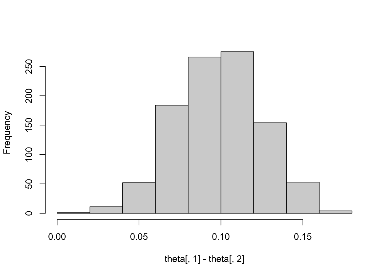

Considers posterior distribution of Obama electoral votes for the 2008 presidential election.

prob.Obama <- function(j){
  p <- with(election.2008, 
            rdirichlet(5000,
          500 * c(M.pct[j], O.pct[j], 
          100 - M.pct[j] - O.pct[j]) / 100 + 1))
  mean(p[, 2] > p[, 1])
}
Obama.win.probs <- sapply(1 : 51, prob.Obama)

sim.election <- function(){
  winner <- rbinom(51, 1, 
              Obama.win.probs)  
  sum(election.2008$EV * winner)         
}

sim.EV <- replicate(1000, sim.election())

hist(sim.EV, min(sim.EV) : max(sim.EV), col="blue")
abline(v=365, lwd=3)  # Obama received 365 votes
text(375, 30, "Actual \n Obama \n total")

4.3 A Bioassay Experiment

Bayesian fitting of a logistic model using data from a dose-response experiment.

x <- c(-0.86, -0.3, -0.05, 0.73)
n <- c(5, 5, 5, 5)
y <- c(0, 1, 3, 5)
data <- cbind(x, n, y)

Traditional logistic model fit.

glmdata <- cbind(y, n - y)
results <- glm(glmdata ~ x, family = binomial)
summary(results)

## 
## Call:
## glm(formula = glmdata ~ x, family = binomial)
## 
## Deviance Residuals: 
##        1         2         3         4  
## -0.17236   0.08133  -0.05869   0.12237  
## 
## Coefficients:
##             Estimate Std. Error z value Pr(>|z|)
## (Intercept)   0.8466     1.0191   0.831    0.406
## x             7.7488     4.8728   1.590    0.112
## 
## (Dispersion parameter for binomial family taken to be 1)
## 
##     Null deviance: 15.791412  on 3  degrees of freedom
## Residual deviance:  0.054742  on 2  degrees of freedom
## AIC: 7.9648
## 
## Number of Fisher Scoring iterations: 7

Illustration of a conditional means prior. When x = -.7, median and 90th percentile of p are (.2,.4). When x = +.6, median and 90th percentile of p are (.8, .95)

a1.b1 <- beta.select(list(p=.5, x=.2),
                    list(p=.9, x=.5))
a2.b2 <- beta.select(list(p=.5, x=.8),
                  list(p=.9, x=.98))

prior <- rbind(c(-0.7, 4.68, 1.12),
            c(0.6, 2.10, 0.74))
data.new <- rbind(data, prior)

Plot prior.

plot(c(-1,1), c(0, 1), type="n", 
     xlab="Dose", ylab="Prob(death)")
lines(-0.7 * c(1, 1), qbeta(c(.25, .75), 
      a1.b1[1], a1.b1[2]), lwd=4)
lines(0.6 * c(1, 1), qbeta(c(.25, .75), 
      a2.b2[1], a2.b2[2]), lwd=4)
points(c(-0.7, 0.6), qbeta(.5, c(a1.b1[1],
          a2.b2[1]), c(a1.b1[2], a2.b2[2])),
         pch=19, cex=2)
text(-0.3, .2, "Beta(1.12, 3.56)")
text(.2, .8, "Beta(2.10, 0.74)")
response <- rbind(a1.b1, a2.b2)
x <- c(-0.7, 0.6)
fit <- glm(response ~ x, family = binomial)

## Warning in eval(family$initialize): non-integer counts in a binomial glm!

curve(exp(fit$coef[1] + fit$coef[2] * x) /
     (1 + exp(fit$coef[1] + fit$coef[2] * x)),
     add=T)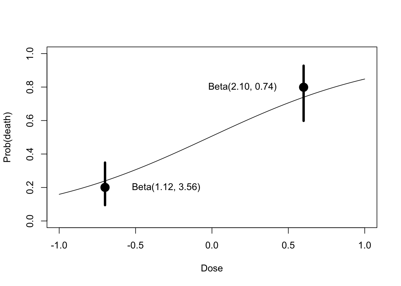

Posterior of regression coefficients.

mycontour(logisticpost, c(-3, 3, -1, 9), data.new,
  xlab="beta0", ylab="beta1")

mycontour(logisticpost, c(-3, 3, -1, 9), data.new,
  xlab="beta0", ylab="beta1")
s <- simcontour(logisticpost, c(-2, 3, -1, 11),
                data.new, 1000)
points(s)

plot(density(s$y), xlab="beta1")

Estimation of LD50 parameter.

theta <- -s$x / s$y
hist(theta, xlab="LD-50", breaks=20,
     xlim = c(-1, 1.5))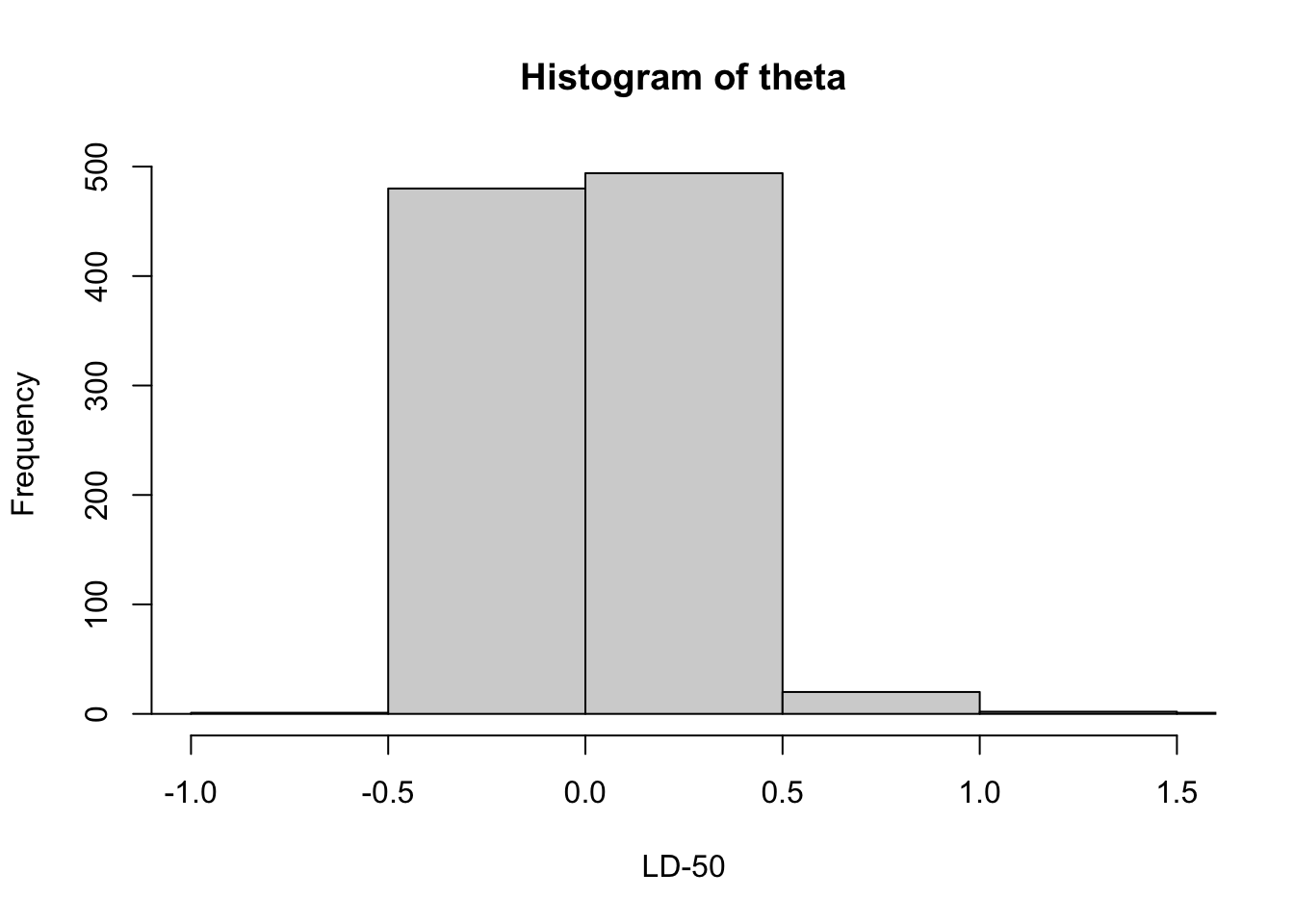

quantile(theta, c(.025, .975))

##       2.5%      97.5% 
## -0.3248469  0.4748061

4.4 Comparing Two Proportions

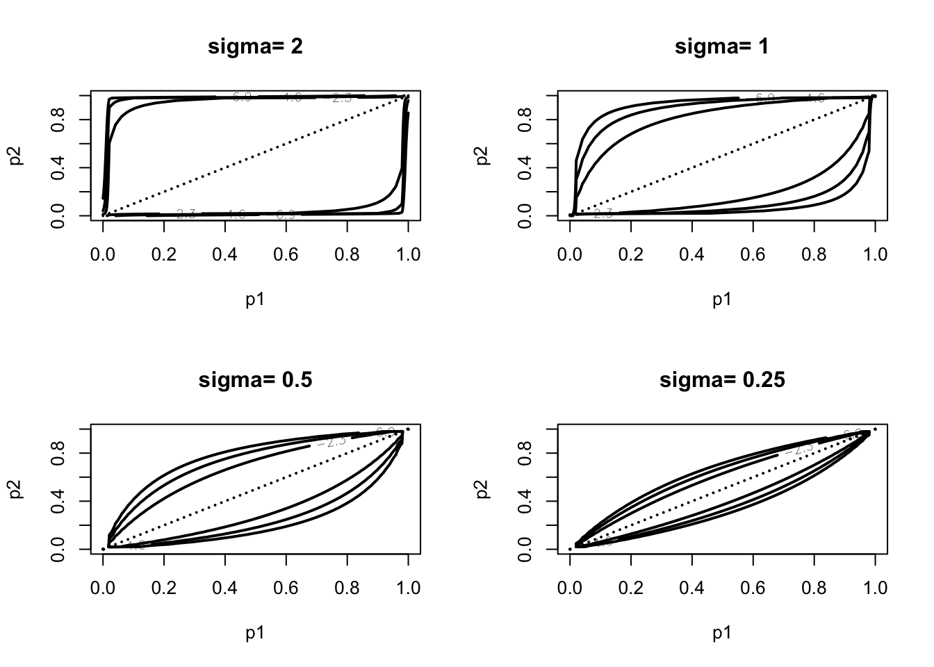
Using Howard’s dependent prior for two proportions. Graph of the prior.

sigma <- c(2, 1, .5, .25)
plo <- .0001; phi <- .9999
par(mfrow=c(2, 2))
for (i in 1:4){
    mycontour(howardprior, 
              c(plo, phi, plo, phi),
              c(1, 1, 1, 1, sigma[i]),
      main=paste("sigma=", as.character(sigma[i])),
      xlab="p1", ylab="p2")
}

Graphs of the posterior.

sigma <- c(2, 1, .5, .25)
par(mfrow=c(2, 2))
for (i in 1:4){
   mycontour(howardprior,
             c(plo, phi, plo, phi),
     c(1 + 3, 1 + 15, 1 + 7, 1 + 5, sigma[i]),
     main=paste("sigma=", as.character(sigma[i])),
     xlab="p1", ylab="p2")
   lines(c(0, 1), c(0, 1))
 }

s <- simcontour(howardprior, c(plo, phi, plo, phi),
   c(1 + 3, 1 + 15, 1 + 7, 1 + 5, 2), 1000)
sum(s$x > s$y) / 1000

## [1] 0.012