Chapter 5 Comparing Proportions

5.1 Packages for example

library(ProbBayes)
library(brms)
library(dplyr)
library(ggplot2)

5.2 Facebook use example

In Chapter 9, we consider the following comparison of proportions example. A sample of students were asked their gender and the average number of times they visited Facebook in a day.

Of \(n_M\) males sampled, \(y_M\) had a high number of Facebook visits, and of \(n_F\) females sampled, \(y_F\) had a high number of visits.

Suppose the data is organized as a data frame as follows:

Gender	Sample_size	Visits
male	\(n_M\)	\(y_M\)
female	\(n_F\)	\(y_F\)

5.3 Sampling model

Suppose we have two independent samples where \(y_M\) is binomial(\(n_M, p_M\)) and \(y_F\) is binomial(\(n_F, p_F\)).

Write the proportions using a logistic model:

\[ \log\left(\frac{p}{1-p}\right) = \beta_0 + \beta_1 I(Gender = Male) \]

Note for females, the logit of \(p_F\) is given by \[ \log\left(\frac{p}{1-p}\right) = \beta_0 \] and for males the logit for \(p_M\) is given by \[ \log\left(\frac{p}{1-p}\right) = \beta_0 + \beta_1 \]

5.4 The data

Here’s the observed data:

fb_data <- data.frame(Gender = c("male", "female"),
                      Sample_Size = c(93, 151),
                      Visits = c(39, 75))

5.5 Priors

In this model, \(\beta_0\) is the logit of the proportion of women who are high Facebook users and \(\beta_1\) represents the difference in the logits of the proportions for men and women.

Assume that you don’t know much about the location of \(\beta_0\), but you believe men and women are similar in their use of Facebook. So you assign a N(0, 31.6) prior to \(\beta_0\) with a high standard deviation, reflecting little knowledge. To reflect the belief that \(\beta_1\) is close to 0, you use a N(0, 0.71) prior.

The get_prior() function lists all parameters to define priors on for this particular model, assigning the result to prior. Then the two components of prior are assigned that reflect the statements above.

(my_prior <- get_prior(family = binomial,
           Visits | trials(Sample_Size) ~ Gender,
           data = fb_data))

##                  prior     class       coef group resp dpar nlpar bound
## 1                              b                                       
## 2                              b Gendermale                            
## 3 student_t(3, 0, 2.5) Intercept

my_prior$prior[3] <- "normal(0, 31.6)"
my_prior$prior[2] <- "normal(0, 0.71)"

5.6 Posterior sampling

Here is the run of brm() where I use the prior specification in my_prior.

fit <- brm(family = binomial,
           Visits | trials(Sample_Size) ~ Gender,
           data = fb_data,
           prior = my_prior,
           iter = 1000,
           refresh = 0)

## Compiling Stan program...

## Start sampling

One obtains the matrix of simulated values of the parameters by the posterior_samples() function.

post <- posterior_samples(fit)
head(post)

##    b_Intercept b_Gendermale      lp__
## 1  0.149825204   -0.3929578 -10.89798
## 2 -0.077477237   -0.1550768 -10.36612
## 3  0.014914205   -0.2591160 -10.32287
## 4 -0.244104208   -0.2079800 -11.39275
## 5 -0.006092644   -0.2035093 -10.36111
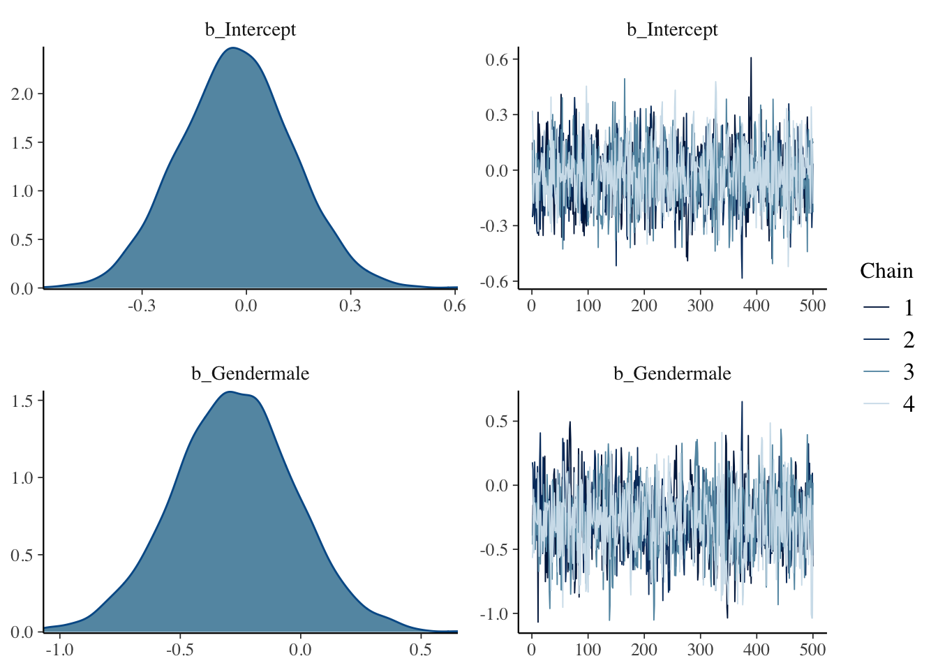
## 6  0.012292753   -0.4538551 -10.53464

The plot() function provides trace plots and density plots of each parameter.

plot(fit)

Posterior summaries are provided by the print() function.

print(fit)

##  Family: binomial 
##   Links: mu = logit 
## Formula: Visits | trials(Sample_Size) ~ Gender 
##    Data: fb_data (Number of observations: 2) 
## Samples: 4 chains, each with iter = 1000; warmup = 500; thin = 1;
##          total post-warmup samples = 2000
## 
## Population-Level Effects: 
##            Estimate Est.Error l-95% CI u-95% CI Rhat Bulk_ESS Tail_ESS
## Intercept     -0.03      0.16    -0.34     0.28 1.00     2198     1576
## Gendermale    -0.28      0.25    -0.78     0.23 1.01     1525     1121
## 
## Samples were drawn using sampling(NUTS). For each parameter, Bulk_ESS
## and Tail_ESS are effective sample size measures, and Rhat is the potential
## scale reduction factor on split chains (at convergence, Rhat = 1).