Chapter 3 Normal Modeling
3.2 Normal sampling model
Assume that \(y_1, ..., y_n\) are a sample from a normal distribution with mean \(\mu\) and standard deviation \(\sigma\).
For a prior, we assume that \(\mu\) and \(\sigma\) are independent where \(\mu\) is assigned a normal prior and \(\sigma\) is assigned a uniform prior on an interval.
3.3 Data and prior
We consider the variable time from the dataset federer_time_to_serve that contains the time to serve for 20 serves of Roger Federer.
We place a weakly informative prior on the parameters. We assume the mean time-to-serve \(\mu\) is N(15, 5) and assume the standard deviation \(\sigma\) is uniform on the interval (0, 20).
3.4 Bayesian fitting
We use the brm() function with the family = gaussian option. Note how the prior is specified by the prior argument.
fit <- brm(data = federer_time_to_serve,
            family = gaussian,
            time ~ 1,
    prior = c(prior(normal(15, 5), class = Intercept),
              prior(uniform(0, 20), class = sigma)),
    iter = 1000, refresh = 0, chains = 4)
## Warning: It appears as if you have specified an upper bounded prior on a parameter that has no natural upper bound.
## If this is really what you want, please specify argument 'ub' of 'set_prior' appropriately.
## Warning occurred for prior
## sigma ~ uniform(0, 20)## Compiling Stan program...## Start samplingOne obtains density plots and trace plots for \(\mu\) and \(\sigma\) by the plot() function.
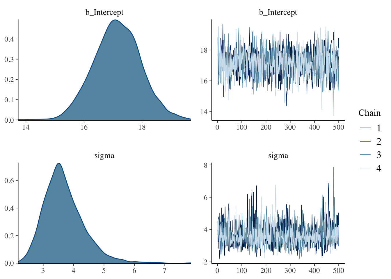
One obtains posterior summaries for each parameter by the summary() function.
##  Family: gaussian
##   Links: mu = identity; sigma = identity
## Formula: time ~ 1
##    Data: federer_time_to_serve (Number of observations: 20)
## Samples: 4 chains, each with iter = 1000; warmup = 500; thin = 1;
##          total post-warmup samples = 2000
##
## Population-Level Effects:
##           Estimate Est.Error l-95% CI u-95% CI Rhat Bulk_ESS Tail_ESS
## Intercept    17.14      0.80    15.58    18.70 1.00     1394     1053
##
## Family Specific Parameters:
##       Estimate Est.Error l-95% CI u-95% CI Rhat Bulk_ESS Tail_ESS
## sigma     3.68      0.66     2.64     5.21 1.00     1137      878
##
## Samples were drawn using sampling(NUTS). For each parameter, Bulk_ESS
## and Tail_ESS are effective sample size measures, and Rhat is the potential
## scale reduction factor on split chains (at convergence, Rhat = 1).
One can obtain a matrix of simulated draws by the posterior_samples() function.
##   b_Intercept    sigma      lp__
## 1    17.69829 3.989865 -57.47744
## 2    17.47939 3.252316 -57.01475
## 3    15.76746 4.781054 -59.40308
## 4    17.62919 4.469536 -58.14521
## 5    16.42508 2.837153 -58.30991
## 6    18.14501 3.504918 -57.70406