Chapter 8 Multilevel Modeling of Means
8.2 Movie Ratings Study
Table 10.1 gives summaries of the ratings for eight different animation movies. The table includes the number of ratings, the mean and the standard deviation of the ratings. The data is contained in the data frame animation_ratings in the ProbBayes package.
8.3 The Multilevel Model
Sampling
Let \(y_{ij}\) denote the rating of the \(i\)th individual for the \(j\)th movie.
We assume that \(y_{ij} \sim N(\mu_j, \sigma)\).
Prior
The parameters \(\mu_1, ..., \mu_8\) represent the mean ratings for the eight movies. Write \[ \mu_j = \beta + \gamma_j \]
The intercept parameter \(\beta\) has a student t distribution with mean 4, scale parameter 2.5, and 3 degrees of freedom.
We assume the effect parameters \(\gamma_1, ..., \gamma_8\) have a normal distribution with mean 0 and standard deviation \(\tau\).
There are two standard deviations, the sampling standard deviation \(\sigma\) and the between-means standard deviation \(\tau\). Each of these standard deviations are given weakly informative student t distributions with mean 0, scale 2.5 and 3 degrees of freedom.
8.4 Bayesian Fitting
The model is fit by use of the brm() function. By default, this function assumes a Gaussian (normal) sampling distribution. The “(1 | movieID)” argument indicates that the \(\mu_1, ..., \mu_8\) have a random distribution.
## Compiling Stan program...## Start sampling## Warning: There were 6 divergent transitions after warmup. Increasing adapt_delta above 0.8 may help. See
## http://mc-stan.org/misc/warnings.html#divergent-transitions-after-warmup## Warning: Examine the pairs() plot to diagnose sampling problemsOne can check the default priors by use of the prior_summary() function.
##                  prior     class      coef   group resp dpar nlpar bound
## 1 student_t(3, 4, 2.5) Intercept
## 2 student_t(3, 0, 2.5)        sd
## 3                             sd           movieId
## 4                             sd Intercept movieId
## 5 student_t(3, 0, 2.5)     sigma
The posterior matrix of simulated draws is available by use of the posterior_samples() function. Below I construct density estimates of the two standard deviation parameters \(\sigma\) (blue) and \(\tau\) (red).
ggplot(posterior_samples(fit),
       aes(sigma)) +
  geom_density(color = "blue") +
  geom_density(aes(sd_movieId__Intercept),
               color = "red")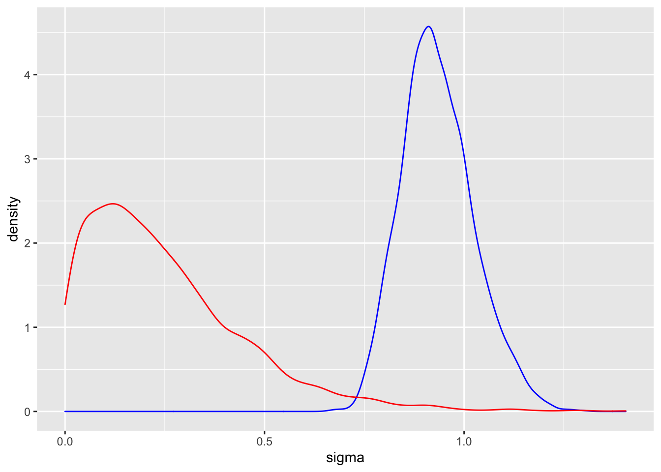
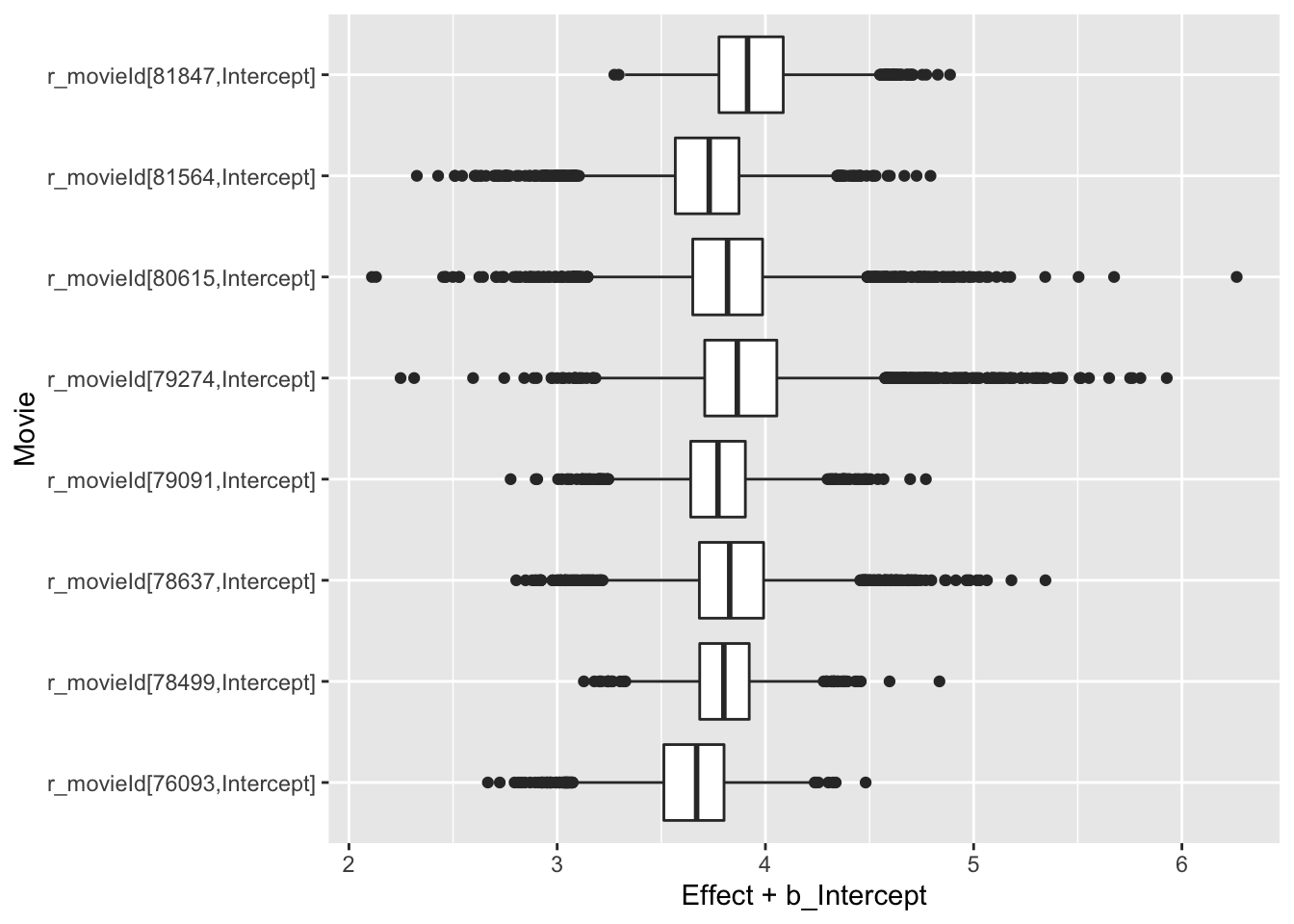
To show the posterior distributions of the means, I reshape the matrix of simulated draws by use of the pivot_longer() function.
posterior_samples(fit) %>%
  pivot_longer('r_movieId[76093,Intercept]':'r_movieId[81847,Intercept]',
               names_to = "Movie",
               values_to = "Effect") -> post
Remember that we represented the movie ratings mean as \(\mu_j = \beta + \gamma_j\). Below are parallel boxplots of the posterior distributions of \(\mu_1, ..., \mu_8\).