Chapter 7 Multilevel Modeling of Proportions
7.2 Hospital Study
Table 10.2 gives the number of cases and number of deaths from heart attacks for 13 hospitals in New York City. This data is contained in the data frame DeathHeartAttackManhattan in the ProbBayes package.
7.3 A Multilevel Model
We consider a different formulation of the hierarchical model described in Section 10.3.
Sampling
We first assume that \(y_j\), the number of deaths for the \(j\)th hospital, is binomial with sample size \(n_j\) and probability \(p_j\). Let \(\theta_j = \log (p_j / (1 - p_j))\) denote the logit for the \(j\)th hospital.
Write \(\theta_j = \beta + \gamma_j\).
Prior
We assume the intercept \(\beta\) has a student t distribution with mean 0, scale parameter 2.5 and 3 degrees of freedom.
We assume \(\gamma_1, ..., \gamma_N\) have a normal distribution with mean 0 and standard deviation \(\sigma\).
The standard deviation \(\sigma\) is assumed to have a t density with mean 0 and standard deviation 3.5.
7.4 Fitting the Bayesian model
We fit the multilevel model using the `brm() function. Note the use of the “family = binomial” argument to indicate the sampling distribution. The “(1 | Hospital)” component indicates that the \(\gamma_j\) have a random distribution.
fit <- brm(data = DeathHeartAttackManhattan,
           family = binomial,
           Deaths | trials(Cases) ~ 1 + (1 | Hospital),
           refresh = 0)
## Compiling Stan program...## Start samplingWe didn’t specify priors, but there are default priors behind the scenes. The prior_summary() function displays the priors.
##                  prior     class      coef    group resp dpar nlpar bound
## 1 student_t(3, 0, 2.5) Intercept
## 2 student_t(3, 0, 2.5)        sd
## 3                             sd           Hospital
## 4                             sd Intercept Hospital
7.5 Posterior summaries of \(\beta\) and \(\sigma\)
The summary() function shows posterior summaries of \(\beta\) (the intercept) and the standard deviation \(\sigma\).
##  Family: binomial
##   Links: mu = logit
## Formula: Deaths | trials(Cases) ~ 1 + (1 | Hospital)
##    Data: DeathHeartAttackManhattan (Number of observations: 13)
## Samples: 4 chains, each with iter = 2000; warmup = 1000; thin = 1;
##          total post-warmup samples = 4000
##
## Group-Level Effects:
## ~Hospital (Number of levels: 13)
##               Estimate Est.Error l-95% CI u-95% CI Rhat Bulk_ESS Tail_ESS
## sd(Intercept)     0.19      0.15     0.01     0.56 1.00      913     1675
##
## Population-Level Effects:
##           Estimate Est.Error l-95% CI u-95% CI Rhat Bulk_ESS Tail_ESS
## Intercept    -2.60      0.11    -2.82    -2.37 1.00     2555     1376
##
## Samples were drawn using sampling(NUTS). For each parameter, Bulk_ESS
## and Tail_ESS are effective sample size measures, and Rhat is the potential
## scale reduction factor on split chains (at convergence, Rhat = 1).
7.6 Posterior summaries of hospital effects
The posterior_samples() function produces a large matrix of simulated draws where the column corresponds to the parameter and the row corresponds to the iteration number.
By use of the pivot_longer() function, I reformat the simulation matrix where there is a new variable Hospital indicating the name of the hospital and Effect is the simulated value of \(\gamma_j\). Also I create a new variable that is the number of the hospital from 1 to 13.
posterior_samples(fit) %>%
pivot_longer(starts_with("r_Hospital"),
names_to = "Hospital",
values_to = "Effect") -> post
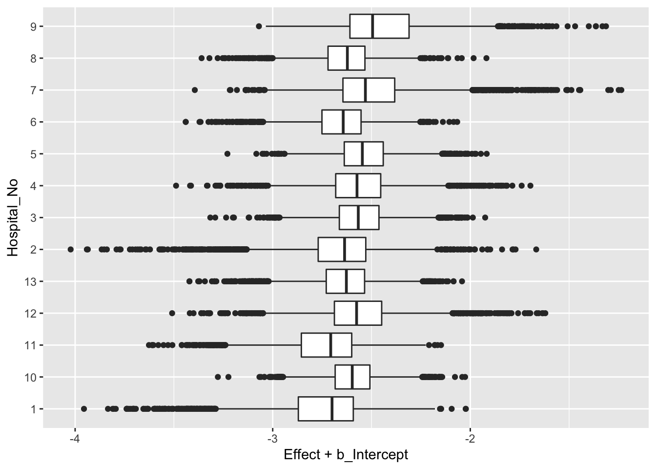
post$Hospital_No <- as.character(as.numeric(factor(post$Hospital)))Below is a graph of the posterior distribution of the parameters {\(\beta + \gamma_j\)} for all 13 hospitals.
These are graphed on the logit scale. By taking the inverse logit function, one could find the posterior distributions of the death rates \(p_1, ..., p_N\).