Chapter 6 Comparing Rates

6.1 Packages for example

library(ProbBayes)
library(brms)
library(dplyr)

6.2 Comparing two Poisson Rates

Suppose we observe two independent samples: \(x_1, ..., x_m\) are a random sample from a Poisson distribution with mean \(\lambda_x\), and \(w_1, ..., w_n\) are a random sample from a Poisson distribution with mean \(\lambda_y\). We are interested in learning about the ratio of Poisson means \[ \theta = \frac{\lambda_x}{\lambda_y} \]

6.3 Write as a log-linear model

Suppose we collect the observations \[ y = c(x_1, ..., x_m, w_1, ..., w_n) \] and let group2 be an indicator variable for the second group. \[ group2 = c(0, 0, ..., 0, 1, 1, ..., 1) \] Then we can represent the model as \[ y_1, ..., y_{m+n} \] independent from Poisson distributions with means \(\lambda_1, ..., \lambda_{m_n}\) where the means follow the log-linear model \[ \log \lambda_j = \beta_0 + \beta_1 group2 \]

In this model, \(\beta_0 = \log \lambda_x\), and \(\beta_0 + \beta_1 = \log \lambda_y\). So \(\beta_1 = \log(\lambda_y) - \log(\lambda_x)\) represents the increase in the means on the log scale.

6.4 The data

We collect web count visits for a number of days stored in the data frame web_visits in the ProbBayes package. The key variables are Day, the day of the week, and Count, the website visit count. We define a new variable Type that is either “weekend” or “weekday”.

We are interested in comparing the mean visit counts for weekdays and weekend days.

web_visits %>% 
  mutate(Type = ifelse(Day %in% 
      c("Fri", "Sat", "Sun"), "weekend", "weekday")) -> web_visits

6.5 Priors

Here we are assume weakly informative priors on the regression parameters \(\beta_0\) and \(\beta_1\).

6.6 Bayesian fitting

fit <- brm(Count ~ Type,
           family = poisson,
           data = web_visits,
           refresh = 0)

## Compiling Stan program...

## Start sampling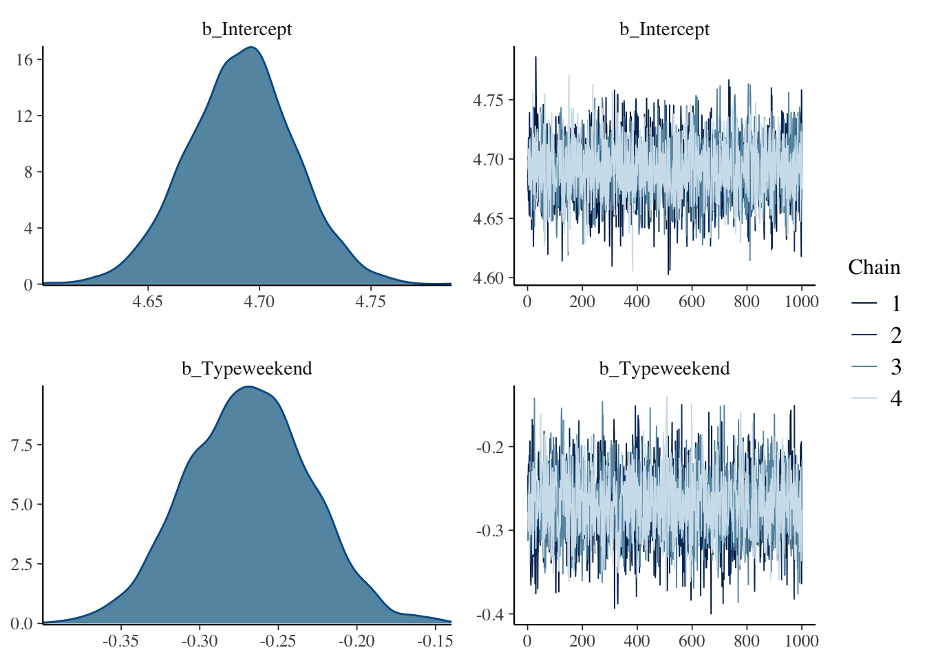

plot(fit)

summary(fit)

##  Family: poisson 
##   Links: mu = log 
## Formula: Count ~ Type 
##    Data: web_visits (Number of observations: 28) 
## Samples: 4 chains, each with iter = 2000; warmup = 1000; thin = 1;
##          total post-warmup samples = 4000
## 
## Population-Level Effects: 
##             Estimate Est.Error l-95% CI u-95% CI Rhat Bulk_ESS Tail_ESS
## Intercept       4.69      0.02     4.64     4.74 1.00     3888     2663
## Typeweekend    -0.27      0.04    -0.35    -0.19 1.00     3292     2805
## 
## Samples were drawn using sampling(NUTS). For each parameter, Bulk_ESS
## and Tail_ESS are effective sample size measures, and Rhat is the potential
## scale reduction factor on split chains (at convergence, Rhat = 1).

sim_draws <- posterior_samples(fit)
head(sim_draws)

##   b_Intercept b_Typeweekend      lp__
## 1    4.683972    -0.3003928 -111.6071
## 2    4.690432    -0.2403990 -111.1721
## 3    4.665176    -0.2213930 -111.6114
## 4    4.683088    -0.2696015 -110.9016
## 5    4.678049    -0.2929583 -111.6562
## 6    4.699903    -0.2566505 -111.0721