Chapter 4 Poisson Modeling

4.1 Packages for example

library(ProbBayes)
library(brms)

4.2 Poisson log-linear model

Here we observe counts \(y_1, ..., y_n\) distributed according to a Poisson distribution with mean \(\lambda\).

Write a model in terms of the logarithm of the mean:

\[ \theta = \log \lambda \]

Complete the model by assigning a \(N(\mu, \sigma)\) prior to the log mean parameter \(\theta\).

4.3 Learning about website counts

In the ProbBayes package, the variable Count in the dataset web_visits contains counts of daily visits to a blog website. We are interested in learning about the mean count of visits \(\lambda\).

We place a N(0, 10) prior on \(\theta = \log \lambda\) reflecting weak prior information about the location of this paramter.

4.4 Bayesian Fitting

In this run of the brm() function, we assume Poisson sampling and a normal prior with mean 0 and standard deviation 10 placed on the log mean \(\theta = \log \lambda\).

fit <- brm(Count ~ 0 + Intercept, 
            data = web_visits,
            family = poisson,
             refresh = 0,
           prior = prior(normal(0, 10), 
                         class = b,
                         coef = "Intercept"))

## Compiling Stan program...

## Start sampling

We confirm the prior with the prior_summary() function.

prior_summary(fit)

##           prior class      coef group resp dpar nlpar bound
## 1                   b                                      
## 2 normal(0, 10)     b Intercept

The summary() function provides summaries of the posterior of \(\theta\).

summary(fit)

##  Family: poisson 
##   Links: mu = log 
## Formula: Count ~ 0 + Intercept 
##    Data: web_visits (Number of observations: 28) 
## Samples: 4 chains, each with iter = 2000; warmup = 1000; thin = 1;
##          total post-warmup samples = 4000
## 
## Population-Level Effects: 
##           Estimate Est.Error l-95% CI u-95% CI Rhat Bulk_ESS Tail_ESS
## Intercept     4.59      0.02     4.55     4.62 1.00     1574     2209
## 
## Samples were drawn using sampling(NUTS). For each parameter, Bulk_ESS
## and Tail_ESS are effective sample size measures, and Rhat is the potential
## scale reduction factor on split chains (at convergence, Rhat = 1).

The posterior_samples() function outputs the posterior simulations of \(\theta\).

post <- posterior_samples(fit)
head(post)

##   b_Intercept      lp__
## 1    4.556476 -136.7185
## 2    4.562960 -136.2752
## 3    4.560979 -136.3987
## 4    4.598670 -135.8759
## 5    4.594855 -135.7515
## 6    4.590376 -135.6570

4.5 Posterior predictive model checks

Actual this is a poor model for these data. One can see that by several posterior predictive checks.

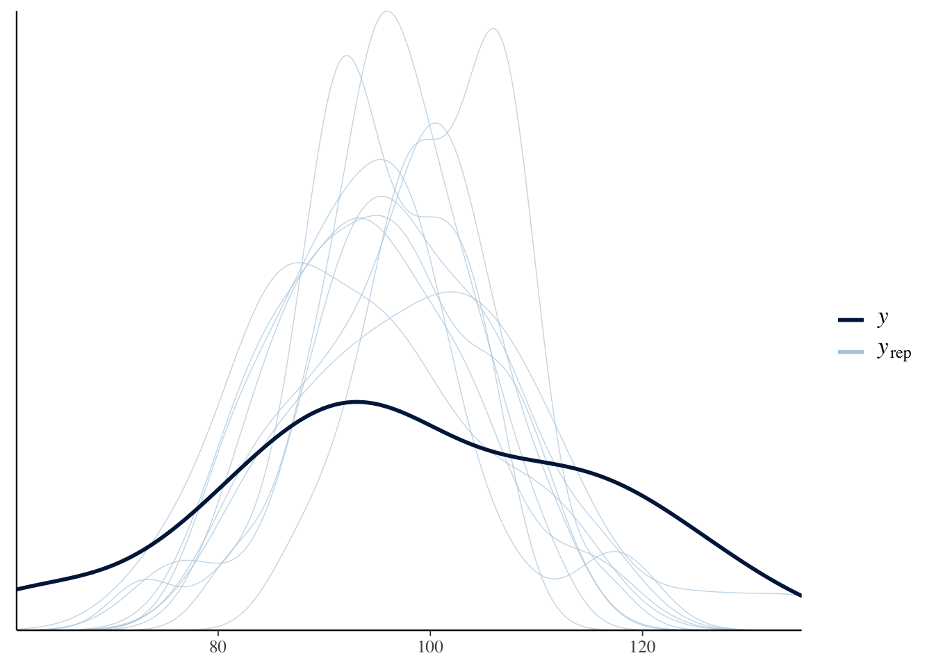
The pp_check() shows density plots of 10 replicated datasets from the posterior predictive distribution. Note that these replicated datasets look different (smaller variation) than the observed data.

pp_check(fit)

## Using 10 posterior samples for ppc type 'dens_overlay' by default.

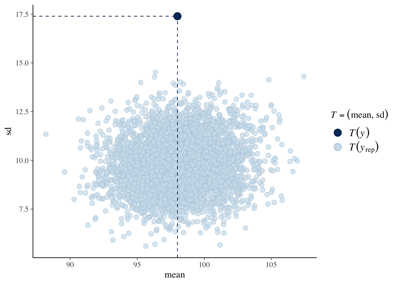
The pp_check() function will implement a posterior predictive check using various checking functions. Here we are using \((\bar y, s)\) as a bivariate checking function. The scatterplot represents values of \((\bar y, s)\) from the simulated predictive distributions and the observed values of \((\bar y, s)\) is displayed. The takeaway is that the observed data has more variation than predicted from the Poisson model.

pp_check(fit, type = "stat_2d")

## Using all posterior samples for ppc type 'stat_2d' by default.