Chapter 10 Federalist Paper Study
10.1 Packages for this example
10.2 Federalist paper data
The data frame federalist_word_study contains frequency use of words for Federalist Papers written by either Alexander Hamilton or James Madison.
We’ll focus on the frequencies of the word “can” in groups of 1000 words written by Hamilton
##                   Name Total word  N         Rate Authorship Disputed
## 65    Federalist No. 1  1622  can  3 0.0018495684   Hamilton       no
## 1526 Federalist No. 11  2511  can  5 0.0019912386   Hamilton       no
## 2437 Federalist No. 12  2171  can  2 0.0009212345   Hamilton       no
## 3125 Federalist No. 13   970  can  4 0.0041237113   Hamilton       no
## 4256 Federalist No. 15  3095  can 14 0.0045234249   Hamilton       no
## 5530 Federalist No. 16  2047  can  1 0.0004885198   Hamilton       no
10.3 The Poisson sampling model
If \(y_i\) represents the count of “can” in the \(i\) group of words, we assume
\[ y_i \sim Poisson(n_i \lambda / 1000), i = 1, ..., N \]
where \(\lambda\) is the true rate of the word among 1000 words.
On log scale, the Poisson mean can be written
\[ \log E(y_i) = \log \lambda + \log(n_i / 1000) \] which can be fit as a generalized linear model with Poisson sampling, log link, intercept model with an offset of \(\log(n_i / 1000)\).
We complete this model by assigning the prior \[ \log \lambda \sim N(0, 2) \]
10.4 Fitting the model
We use the `brm() function with “family = poisson”, specifying the offset “N”, and specifying the prior by use of the “prior” argument.
fit <- brm(data = d, family = poisson,
    N ~ offset(log(Total / 1000)) + 1,
    prior = c(prior(normal(0, 2),
                    class = Intercept)),
              refresh = 0
    )
## Compiling Stan program...## Start samplingWe display summaries of the posterior for \(\lambda\).
## Family: poisson
## Links: mu = log
## Formula: N ~ offset(log(Total/1000)) + 1
## Data: d (Number of observations: 49)
## Samples: 4 chains, each with iter = 2000; warmup = 1000; thin = 1;
## total post-warmup samples = 4000
##
## Population-Level Effects:
## Estimate Est.Error l-95% CI u-95% CI Rhat Bulk_ESS Tail_ESS
## Intercept 0.97 0.06 0.86 1.09 1.00 1602 1974
##
## Samples were drawn using sampling(NUTS). For each parameter, Bulk_ESS
## and Tail_ESS are effective sample size measures, and Rhat is the potential
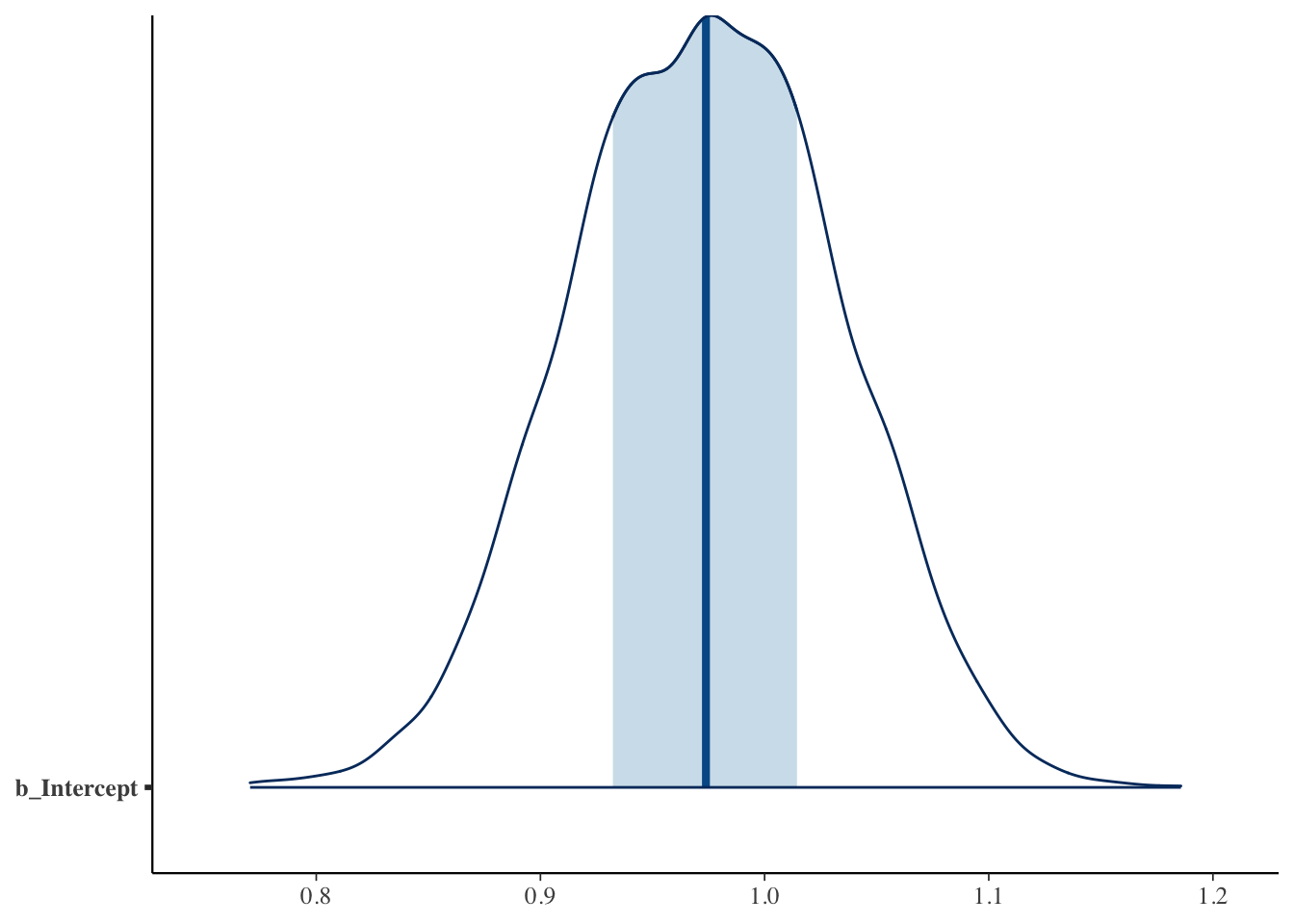
## scale reduction factor on split chains (at convergence, Rhat = 1).We save post as a matrix of simulated draws.
The function mcmc_areas() displays a density estimate of the simulated draws and shows the location of a 50% probability interval.
10.5 Model checking
To check if the Poisson sampling model is appropriate we illustrate several posterior predictive checks.
Here we display density estimates for 10 replicated samples from the posterior predictive distribution of \(y\) and overlay the observed values as a dark line.
## Using 10 posterior samples for ppc type 'dens_overlay' by default.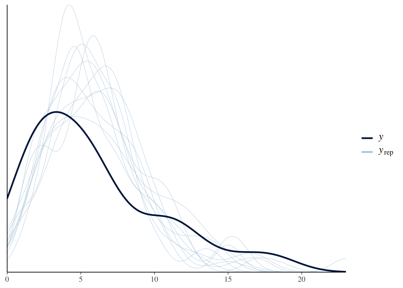
Here we use \((\bar y, s_y)\) as a checking function. The scatterplot represents values of \((\bar y, s_y)\) from the posterior predictive distribution of replicated data, and the observed value of \((\bar y, s_y)\) is shown as a dot.
## Using all posterior samples for ppc type 'stat_2d' by default.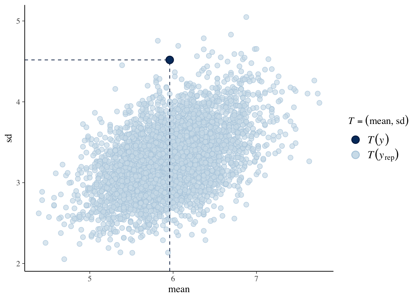
The takeaway is that the observed data shows more variability than predicted from the Poisson sampling model.
10.6 Negative binomial sampling
One way to handle the extra variability is to assume that the \(y_i\) have a negative binomial distribution. (See the text for details.)
Here we outline the code for fitting this model.
We fit the model with the brm() function with the “family = negbinomial” option.
## Compiling Stan program...## Start samplingHere I can checking on the default priors used by brm:
##                    prior     class coef group resp dpar nlpar bound
## 1 student_t(3, 1.6, 2.5) Intercept
## 2      gamma(0.01, 0.01)     shape
Here are the posterior summaries.
##  Family: negbinomial
##   Links: mu = log; shape = identity
## Formula: N ~ offset(log(Total/1000)) + 1
##    Data: d (Number of observations: 49)
## Samples: 4 chains, each with iter = 2000; warmup = 1000; thin = 1;
##          total post-warmup samples = 4000
##
## Population-Level Effects:
##           Estimate Est.Error l-95% CI u-95% CI Rhat Bulk_ESS Tail_ESS
## Intercept     1.00      0.10     0.81     1.19 1.00     3457     2694
##
## Family Specific Parameters:
##       Estimate Est.Error l-95% CI u-95% CI Rhat Bulk_ESS Tail_ESS
## shape     3.28      1.10     1.75     5.97 1.00     3450     2535
##
## Samples were drawn using sampling(NUTS). For each parameter, Bulk_ESS
## and Tail_ESS are effective sample size measures, and Rhat is the potential
## scale reduction factor on split chains (at convergence, Rhat = 1).
I save the posterior samples in the data frame post.
I try the same posterior predictive checks as before. The message is that the negative binomial sampling model is a better fit to these data.
## Using 10 posterior samples for ppc type 'dens_overlay' by default.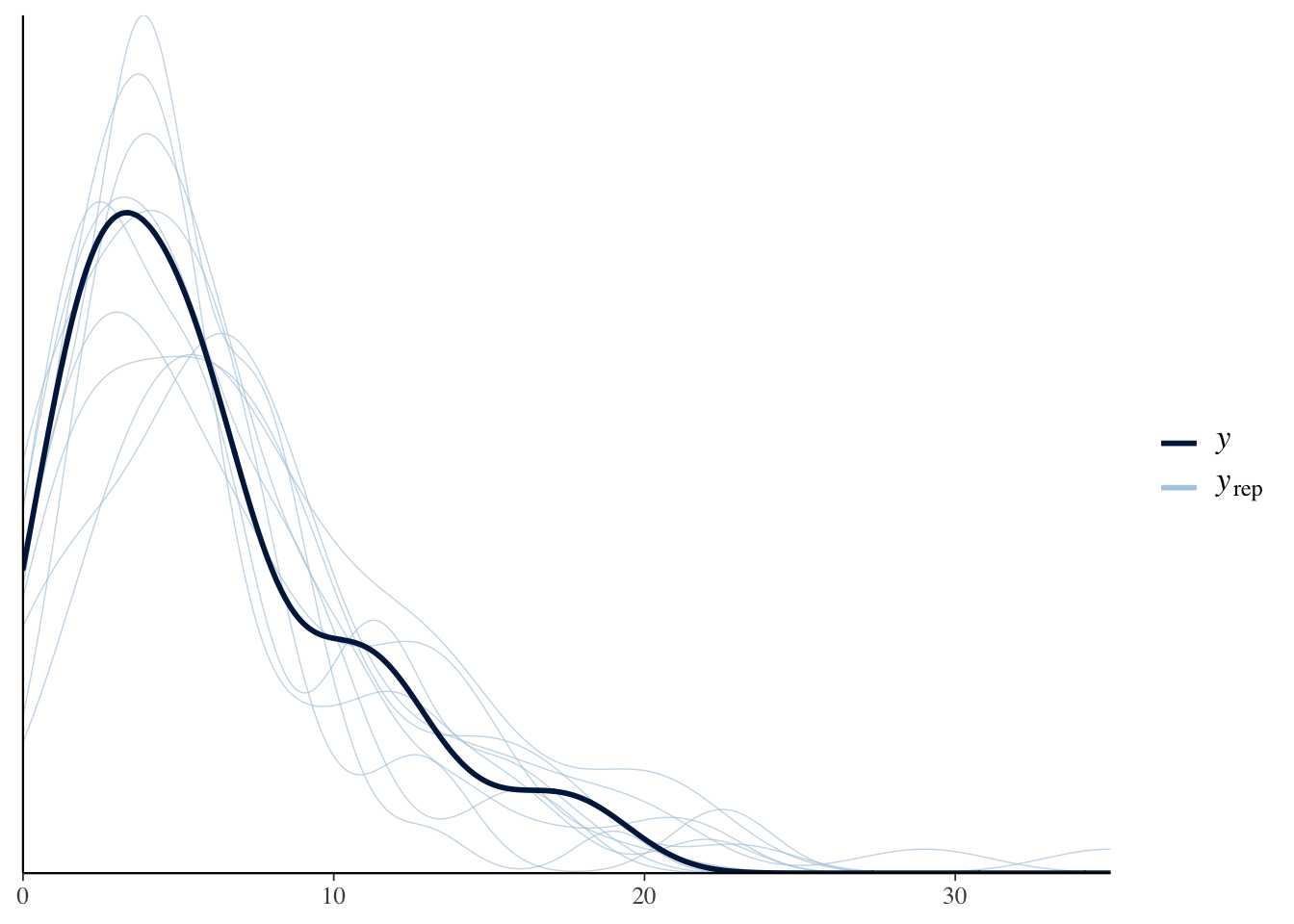
## Using all posterior samples for ppc type 'stat_2d' by default.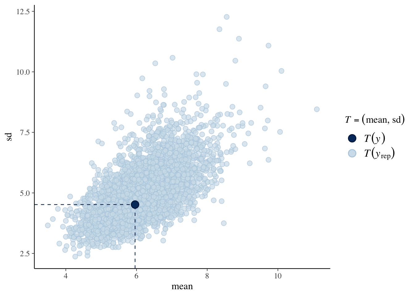
10.7 Comparing use of a word
Next we compare Madison and Hamilton use of the word “can”. The data frame d2 contains only the word data for the essays that were known to be written by Hamilton or Madison.
Here I fit a regression model for the mean use of “can”, where the one predictor is the categorical variable “Authorship”.
fit_nb <- brm(data = d2, family = negbinomial,
           N ~ offset(log(Total / 1000)) +
          Authorship ,
           refresh = 0)
## Compiling Stan program...## Start samplingBy summarizing the fit, we can see if the two authors differ in their use of the word “can” in their writings.
##  Family: negbinomial
##   Links: mu = log; shape = identity
## Formula: N ~ offset(log(Total/1000)) + Authorship
##    Data: d2 (Number of observations: 74)
## Samples: 4 chains, each with iter = 2000; warmup = 1000; thin = 1;
##          total post-warmup samples = 4000
##
## Population-Level Effects:
##                   Estimate Est.Error l-95% CI u-95% CI Rhat Bulk_ESS Tail_ESS
## Intercept             1.00      0.09     0.82     1.19 1.00     3486     2799
## AuthorshipMadison    -0.08      0.16    -0.40     0.25 1.00     3265     2711
##
## Family Specific Parameters:
##       Estimate Est.Error l-95% CI u-95% CI Rhat Bulk_ESS Tail_ESS
## shape     3.84      1.12     2.23     6.48 1.00     3497     2824
##
## Samples were drawn using sampling(NUTS). For each parameter, Bulk_ESS
## and Tail_ESS are effective sample size measures, and Rhat is the potential
## scale reduction factor on split chains (at convergence, Rhat = 1).