Chapter 11 Multilevel Regression

11.1 Packages for example

library(tidyverse)
library(brms)

11.2 Some baseball data

The function get_onbase_data() function collects on-base data for all players born in the year 1977 who have had at least 1000 career plate appearances.

source("get_onbase_data.R")
d78 <- get_onbase_data(1977, 1000)

## `summarise()` ungrouping output (override with `.groups` argument)

## `summarise()` regrouping output by 'playerID' (override with `.groups` argument)

unique(d78$nameLast)

##  [1] "Beltran"    "Bergeron"   "Bigbie"     "Bloomquist" "Byrd"      
##  [6] "Caruso"     "Chavez"     "Davis"      "Ellis"      "Everett"   
## [11] "Fukudome"   "Furcal"     "Gerut"      "Gibbons"    "Gonzalez"  
## [16] "Hafner"     "Hinske"     "Hudson"     "Inge"       "Jimenez"   
## [21] "Jones"      "Monroe"     "Munson"     "Nieves"     "Overbay"   
## [26] "Pierre"     "Punto"      "Quinlan"    "Redman"     "Roberts"   
## [31] "Ross"       "Rowand"     "Sanchez"    "Thames"     "Tyner"     
## [36] "Wigginton"  "Wilkerson"  "Wilson"

11.3 Quadratic aging model

Let \(y_{ij}\) denote the number of on-base events in \(n_{ij}\) opportunities (plate appearances) of the \(i\)th batter in the \(j\)th season. Assume that \(y_{ij}\) is binomial with sample size \(n_{ij}\) and probability of success \(p_{ij}\).

Assume that the on-base probabilities for the \(i\)th player satisfy the logistic model \[ \log \left(\frac{p_{ij}}{1 - p_{ij}}\right) = \beta_{i0} + \beta_{i1} D_{ij} + \beta_{i2} D_{ij}^2 \] where \(D_{ij} = x_{ij} - 30\), \(x_{ij}\) is the age of the \(i\)th player in the \(j\)th season.

11.4 Multilevel Prior

The \(i\)th player’s trajectory is described by the regression vector \(\beta_i = (\beta_{i0}, \beta_{i1}, \beta_{i2})\). We place a two-stage prior on the trajectories \(\beta_1, ..., \beta_N\):

\(\beta_1, ..., \beta_N\) are a sample from a multivariate normal density with mean \(\beta\) and variance-covariance matrix \(\Sigma\).
The second-stage parameters \(\beta\) and \(\Sigma\) are independent with weakly informative priors.

11.5 Bayesian fitting

The fitting of this model is done using the brm() function.

fit <- brm(OB | trials(PA) ~ AgeD + I(AgeD ^ 2) +
             (AgeD + I(AgeD ^  2) | Player),
           data = filter(d78, PA > 0),
           family = binomial("logit"),
           refresh = 0)

## Compiling Stan program...

## Start sampling

I find posterior means of the fitted trajectories for all players.

Player_Fits <- coef(fit)$Player[, "Estimate", ] %>% 
  as.data.frame() %>% 
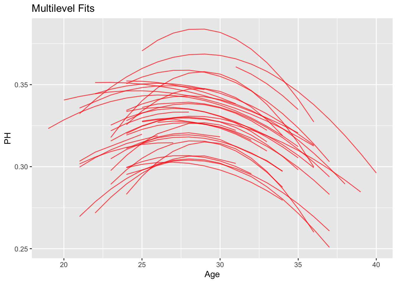
    mutate(Player = 1:max(d78$Player))

d78 <- inner_join(d78, Player_Fits, by = "Player")

d78 %>% 
  mutate(PH = plogis(Intercept + AgeD.y * AgeD.x +
                       IAgeDE2 * AgeD.x ^ 2)) -> d78

ggplot(d78, aes(Age, PH, group = Player)) +
  geom_line(color = "red", alpha = 0.7) +
  ggtitle("Multilevel Fits")

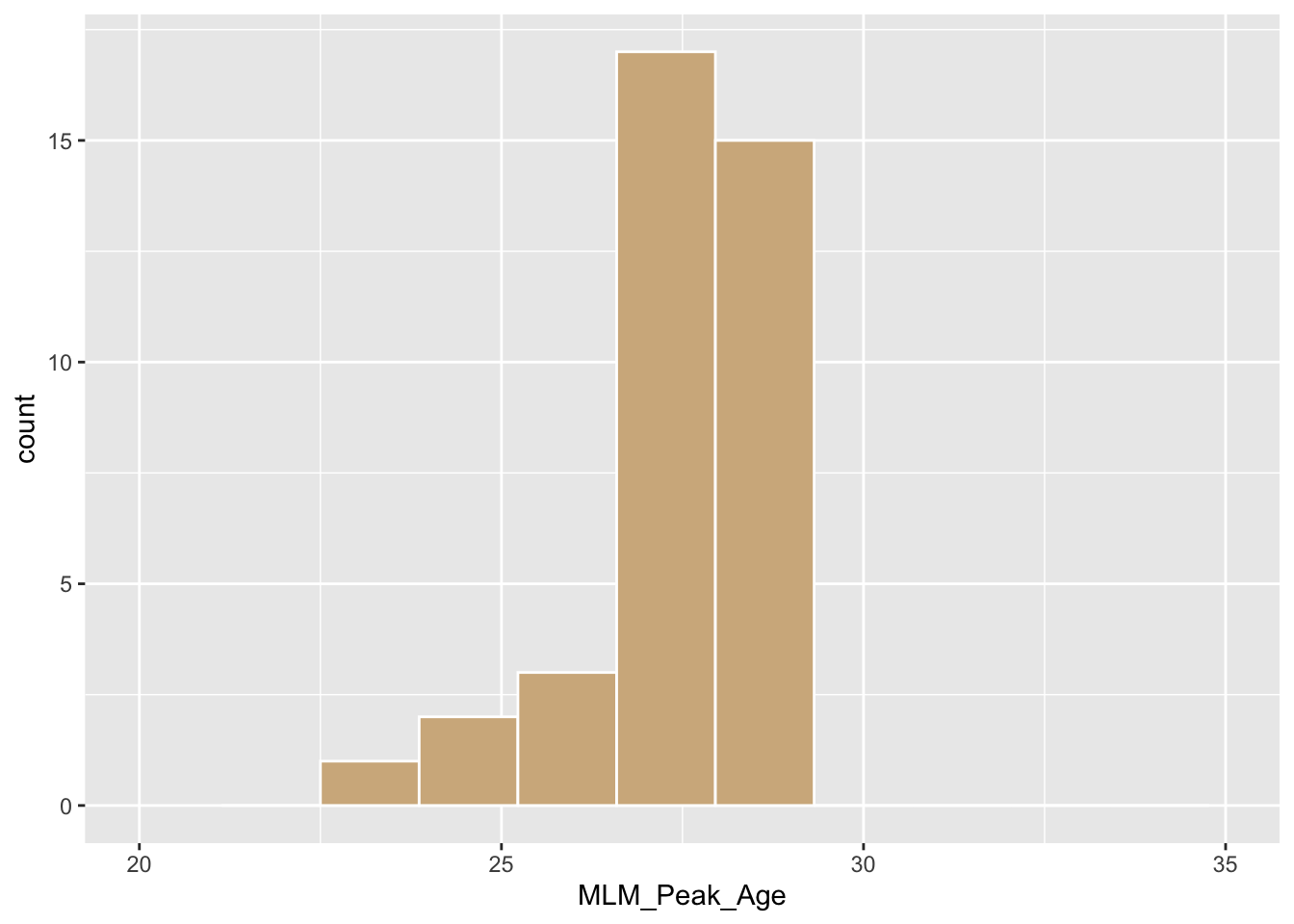
For a given player, define the peak age \[ Age_j = 30 - \frac{\beta_{j1}}{2 \beta_{j2}}. \] the age at which the player achieves peak performance.

The following graph shows the posterior distributions of the peak ages for all players.

d78  %>% group_by(Player) %>% 
  summarize(b0 = first(Intercept),
            b1 = first(AgeD.y),
            b2 = first(IAgeDE2)) %>% 
  mutate(MLM_Peak_Age = 30 - b1 / 2 / b2)  %>% 
  ggplot(aes(MLM_Peak_Age)) +
  geom_histogram(bins = 12, 
                 color = "white", fill = "tan") +
  xlim(20, 35)

## `summarise()` ungrouping output (override with `.groups` argument)

## Warning: Removed 2 rows containing missing values (geom_bar).